Apache Phoenix – an SQL Driver for HBase


Introduction

HBase is one of the most popular NoSQL databases, it is available in all major Hadoop distributions and also part of AWS Elastic MapReduce as an additional application. Out of the box it has its own data model operations such as Get, Put, Scan and Delete and it does not offer SQL-like capabilities, as oppose to, for instance, Cassandra query language, CQL.
Apache Phoenix is a SQL layer on top of HBase to support the most common SQL-like operations such as CREATE TABLE, SELECT, UPSERT, DELETE, etc. Originally it was developed by Salesforce.com engineers for internal use and was open sourced. In 2013 it became an Apache incubator project.

Architecture

We have covered HBase in more detail in this article. Just a quick recap: HBase architecture is based on three key components: HBase Master server, HBase Region Servers and Zookeeper.

HBase-Architecture

The client needs to find the RegionServers in order to work with the data stored in HBase. In essence, regions are the basic elements for distributing tables across the cluster. In order to find the Region servers, the client first will have to talk to Zookeeper.

HBase-Lookup

The key elements in the HBase datamodel are tables, column families, columns and rowkeys. The tables are made of columns and rows. The individual elements at the column and row intersections (cells in HBase term) are version based on timestamp. The rows are identified by rowkeys which are sorted – these rowkeys can be considered as primary keys and all the data in the table can be accessed via them.

The columns are grouped into column families; at table creation time you do not have to specify all the columns, only the column families. Columns have a prefix derived from the column family and its own qualifier,a column name looks like this: ‘contents:html’.

As we have seen, HBase classic data model is not designed with SQL in mind. Under the hood it is a sorted multidimensional Map. That is where Phoenix comes to the rescue; it offers a SQL skin on HBase. Phoenix is implemented as a JDBC driver. From architecture perspective a Java client using JDBC can be configured to work with Phoenix Driver and can connect to HBase using SQL-like statements. We will demonstrate how to use SQuirreL client, a popular Java-based graphical SQL client together with Phoenix.

Getting Started with Phoenix

You can download Phoenix from Apache download site. Different Phoenix versions are compatible with different HBase versions, so please, read Phoenix documentation to ensure you have the correct setup. In our tests we used Phoenix 3.0.0 with HBase 0.94, the Hadoop distribution was Cloudera CDH4.4 with Hadoop v1.. The Phoenix package contains both Hadoop version 1 and version 2 drivers for the clients so we had to use the appropriate Hadoop-1 files, see the details later on when talking about SQuirreL client.

Once you unzipped the downloaded Phoenix package, you need to copy the relevant Phoenix jar files to the HBase region servers in order to ensure that the Phoenix client can communicate with them, otherwise you may get an error message saying that the client and server jars are not compatible.

$ cd ~/phoenix/phoenix-3.0.0-incubating/common
$ cp phoenix-3.0.0-incubating-client-minimal.jar  /usr/lib/hbase/lib
$ cp phoenix-core-3.0.0-incubating.jar /usr/lib/hbase/lib

After you copied the jar files to the region servers, we had to restart them.

Phoenix provides a command line tool called sqlline – it is a utility written in Python. Its functionality is similar to Oracle SQLPlus or MySQL command line tools; not too sophisticated but does the job for simply use cases.

Before you start using sqlline, you can create a sample database table, populate it and run some simple queries as follows:

$ cd ~/phoenix/phoenix-3.0.0.0-incubating/bin
$ ./psql.py localhost ../examples/web_stat.sql ../examples/web_stat.csv ../examples/web_stat_queries.sql

This will run a CREATE TABLE statement:

CREATE TABLE IF NOT EXISTS WEB_STAT (
     HOST CHAR(2) NOT NULL,
     DOMAIN VARCHAR NOT NULL,
     FEATURE VARCHAR NOT NULL,
     DATE DATE NOT NULL,
     USAGE.CORE BIGINT,
     USAGE.DB BIGINT,
     STATS.ACTIVE_VISITOR INTEGER
     CONSTRAINT PK PRIMARY KEY (HOST, DOMAIN, FEATURE, DATE)
);

Then load the data stored in the web_stat CSV file:

NA,Salesforce.com,Login,2013-01-01 01:01:01,35,42,10
EU,Salesforce.com,Reports,2013-01-02 12:02:01,25,11,2
EU,Salesforce.com,Reports,2013-01-02 14:32:01,125,131,42
NA,Apple.com,Login,2013-01-01 01:01:01,35,22,40
NA,Salesforce.com,Dashboard,2013-01-03 11:01:01,88,66,44
...

And the run a few sample queries on the table, e.g.:

-- Average CPU and DB usage by Domain
SELECT DOMAIN, AVG(CORE) Average_CPU_Usage, AVG(DB) Average_DB_Usage 
FROM WEB_STAT 
GROUP BY DOMAIN 
ORDER BY DOMAIN DESC;

Now you can connect to HBase using sqlline:

$ ./sqlline.py localhost
[cloudera@localhost bin]$ ./sqlline.py localhost
..
Connecting to jdbc:phoenix:localhost
Driver: org.apache.phoenix.jdbc.PhoenixDriver (version 3.0)
Autocommit status: true
Transaction isolation: TRANSACTION_READ_COMMITTED
..
Done
sqlline version 1.1.2
0: jdbc:phoenix:localhost> select count(*) from web_stat;
+------------+
|  COUNT(1)  |
+------------+
| 39         |
+------------+
1 row selected (0.112 seconds)
0: jdbc:phoenix:localhost> select host, sum(active_visitor) from web_stat group by host;
+------+---------------------------+
| HOST | SUM(STATS.ACTIVE_VISITOR) |
+------+---------------------------+
| EU   | 698                       |
| NA   | 1639                      |
+------+---------------------------+
2 rows selected (0.294 seconds)
0: jdbc:phoenix:localhost>

Using SQuirreL with Phoenix

If you prefer to use a graphical SQL client with Phoenix, you can download e.g. SQuirreL from here. After that the first step is to copy the appropriate Phoenix driver jar file to SQuirreL lib directory:

$ cd ~/phoenix
$ cp phoenix-3.0.0-incubating/hadoop-1/phoenix-3.0.0.-incubatibg-client.jar ~/squirrel/lib

Now you are ready to configure the JDBC driver in SQuirreL client, as shown in the picture below:

Squirrel-1

Then you can connect to Phoenix using the appropriate connect string (jdbc:phoenix:localhost in our test scenario):

Squirrel-2

Once connected, you can start executing your SQL queries:
Squirrel-3

Phoenix on Amazon Web Services – AWS Elastic MapReduce with Phoenix

You can also use Phoenix with AWS Elastic MapReduce. When you create a cluster, you need to specify Apach Hadoop version, then configure HBase as additional application and define the bootsrap action to load Phoenix onto your AWS EMR cluster. See the details below in the pictures:

AWS-EMR-3

AWS-EMR-5

Once the cluster is running, you can login to the master node using ssh and check your Phoenix configuration.
AWS-EMR-9

Conclusion

SQL is one of the most popular languages used by data scientists and it is likely to remain so. With the advent of Big Data and NoSQL databases the volume, variety and velocity of the data have significantly increased but still the demand for traditional, well-known languages to process them did not change too much. SQL on Hadoop solutions are gaining momentum. Apache Phoenix is interesting open source player to offer SQL layer on top of HBase.

Apache Spark – a Fast Big Data Analytics Engine


Introduction

There are different approaches in big data world to make Hadoop more suitable for ad-hoc, interactive queries and iterative data processing. As it is very well known, Hadoop MapReduce framework is primarily designed for batch processing and that makes it less suitable for ad-hoc data exploration, machine learning processes and the like. Big data vendors are trying to address this challenge by replacing MaReduce with alternatives. In case of SQL on Hadoop, there are various initiatives; Cloudera Impala, Pivotal HAWQ or Hortonworks Stinger initiative that aims to improve Hive performance significantly.

Apache Spark is another increasingly popular alternative to replace MapReduce with a more performant execution engine but still use Hadoop HDFS as storage engine for large data sets.

Spark Architecture

From architecture perspective Apache Spark is based on two key concepts; Resilient Distributed Datasets (RDD) and directed acyclic graph (DAG) execution engine. With regards to datasets, Spark supports two types of RDDs: parallelized collections that are based on existing Scala collections and Hadoop datasets that are created from the files stored on HDFS. RDDs support two kinds of operations: transformations and actions. Transformations create new datasets from the input (e.g. map or filter operations are transformations), whereas actions return a value after executing calculations on the dataset (e.g. reduce or count operations are actions).
The DAG engine helps to eliminate the MapReduce multi-stage execution model and offers significant performance improvements.

Spark-Architecture
Figure 1: Spark Architecture

Installing Spark

Spark is written in Scala so before you install Spark, you need to install Scala. Scala binaries can be downloaded from http://www.scala-lang.org.

$ wget http://www.scala-lang.org/files/archive/scala-2.10.4.tgz
$ tar xvf scala-2.10.4.tgz 
$ ln -s scala-2.10.4 scala
$ vi .bashrc
export SCALA_HOME=/home/istvan/scala
export PATH=$SCALA_HOME/bin:$PATH

You can validate your Scala installation by running Scala REPL (Scala command line interpreter), below is an example how to execute the classic HelloWorld program from Scala:

$ scala
Welcome to Scala version 2.10.4 (Java HotSpot(TM) 64-Bit Server VM, Java 1.6.0_32).
Type in expressions to have them evaluated.
Type :help for more information.

scala> object HelloWorld {
     |     def main(args: Array[String]) {
     |         println("Hello, world!")
     |     }
     | }
defined module HelloWorld

scala> HelloWorld.main(null)
Hello, world!

Then you can download Spark binaries from http://spark.apache.org/downloads.html. There are a couple of pre-compiled versions depending on your Hadoop distribution; we are going to use Spark binaries built for Cloudera CDH4 distribution.

$ wget http://d3kbcqa49mib13.cloudfront.net/spark-0.9.0-incubating-bin-cdh4.tgz
$ tar xvf spark-0.9.0-incubating-bin-cdh4.tgz 
$ ln -s spark-0.9.0-incubating-bin-cdh4 spark

Using Spark shell

Now we are ready to run Spark shell which is a command line interpreter for Spark:

$ bin/spark-shell
14/03/31 15:54:51 INFO HttpServer: Using Spark's default log4j profile: org/apache/spark/log4j-defaults.properties
14/03/31 15:54:51 INFO HttpServer: Starting HTTP Server
Welcome to
      ____              __
     / __/__  ___ _____/ /__
    _\ \/ _ \/ _ `/ __/  '_/
   /___/ .__/\_,_/_/ /_/\_\   version 0.9.0
      /_/

Using Scala version 2.10.3 (Java HotSpot(TM) 64-Bit Server VM, Java 1.6.0_32)
Type in expressions to have them evaluated.
Type :help for more information.
....
14/03/31 15:54:59 INFO HttpServer: Starting HTTP Server
...
Created spark context..
Spark context available as sc.

scala>

In our example we are going to process Apache weblogs that support the common logfile format having the following fields: hostname, timestamp, request, HTTP status code and number of bytes. The test file that we are using in this example is based on the public NASA weblog from 1995 August, see http://ita.ee.lbl.gov/html/contrib/NASA-HTTP.html. The file was cleaned and modified to support tab separated format.

Let us assume that you want to count how many hits the NASA web server got in August, 1995. In order to get the result, you can run the following commands in spark-shell:

Spark context available as sc.

scala> val accessLog = sc.textFile("hdfs://localhost/user/cloudera/weblog/NASA_access_log_Aug95")
14/03/31 16:18:16 INFO MemoryStore: ensureFreeSpace(82970) called with curMem=0, maxMem=311387750
14/03/31 16:18:16 INFO MemoryStore: Block broadcast_0 stored as values to memory (estimated size 81.0 KB, free 296.9 MB)
accessLog: org.apache.spark.rdd.RDD[String] = MappedRDD[1] at textFile at :12

scala> accessLog.count()
14/03/31 16:18:24 INFO FileInputFormat: Total input paths to process : 1
14/03/31 16:18:24 INFO SparkContext: Starting job: count at :15
14/03/31 16:18:24 INFO DAGScheduler: Got job 0 (count at :15) with 2 output partitions (allowLocal=false)
...
14/03/31 16:18:26 INFO HadoopRDD: Input split: hdfs://localhost/user/cloudera/weblog/NASA_access_log_Aug95:134217728+27316431
..
14/03/31 16:18:26 INFO SparkContext: Job finished: count at :15, took 2.297566932 s
res0: Long = 1569898

The first command creates an RDD from the NASA Apache access log stored on HDFS (hdfs://localhost/user/cloudera/weblog/NASA_access_log_Aug95). The second command (an action executed on the accessLog RDD) will count the number of lines in the file. Note that the execution time is around 2 seconds.

If you are interested to know how many requests were initiated from one particular server (e.g. beta.xerox.com in our example), you need to execute a filter operation and then you run count action on the filtered dataset, see:

scala> val filteredLog = accessLog.filter(line => line.contains("beta.xerox.com"))

filteredLog: org.apache.spark.rdd.RDD[String] = FilteredRDD[2] at filter at :14

scala> filteredLog.count()
14/03/31 16:19:35 INFO SparkContext: Starting job: count at :17
14/03/31 16:19:35 INFO DAGScheduler: Got job 1 (count at :17) with 2 output partitions (allowLocal=false)
...
14/03/31 16:19:35 INFO Executor: Running task ID 2
...
14/03/31 16:19:35 INFO HadoopRDD: Input split: hdfs://localhost/user/cloudera/weblog/NASA_access_log_Aug95:0+134217728
14/03/31 16:19:36 INFO Executor: Serialized size of result for 2 is 563
1...
14/03/31 16:19:36 INFO HadoopRDD: Input split: hdfs://localhost/user/cloudera/weblog/NASA_access_log_Aug95:134217728+27316431
...
14/03/31 16:19:37 INFO DAGScheduler: Stage 1 (count at :17) finished in 1.542 s
14/03/31 16:19:37 INFO SparkContext: Job finished: count at :17, took 1.549706892 s
res1: Long = 2318

You can also execute more complex logic and define your own functions, thanks to Scala language capabilities. Let us assume that we need to calculate the total number of bytes generated by the given NASA web server in August, 1995. The number of bytes is the last (5th) field in the lines in the weblog file and unfortunately, there are cases when the field is ‘-‘, not an integer value as it would be expected. The standard toInt Scala String function throws an exception if you want to convert a non-numeric value into Integer. Thus we need to be able to identify whether a given string is a number or not and if not, we need to return 0. This requires a custom function (convertToInt) that will extend the standard String Scala class and will be made available for the String data type. Then we can use this custom function and the Spark standard RDD operations to calculate the total number of  bytes generated by the NASA webserver.

scala> def isNumeric(input: String): Boolean = input.forall(_.isDigit)
isNumeric: (input: String)Boolean


scala> class StringHelper(s:String) {
     |    def convertToInt():Int = if (isNumeric(s)) s.toInt else 0
     | }
defined class StringHelper


scala> implicit def stringWrapper(str: String) = new StringHelper(str)
warning: there were 1 feature warning(s); re-run with -feature for details
stringWrapper: (str: String)StringHelper


scala> "123".convertToInt
res2: Int = 123

scala> "-".convertToInt
res4: Int = 0

scala> accessLog.map(line=>line.split("\t")).map(line=>line(4).convertToInt).sum
14/04/01 13:12:39 INFO SparkContext: Starting job: sum at :21
14/04/01 13:12:39 INFO DAGScheduler: Got job 2 (sum at :21) with 2 output partitions (allowLocal=false)
...
14/04/01 13:12:40 INFO HadoopRDD: Input split: hdfs://localhost/user/cloudera/weblog/NASA_access_log_Aug95:0+134217728
... 
14/04/01 13:12:45 INFO SparkContext: Job finished: sum at :21, took 5.53186208 s
res4: Double = 2.6828341424E10

As you can see, the result is 26,8GB and the calculation was executed in 5.5 seconds.

Programming Spark

In addition to spark-shell that can be used to execute operations interactively, you can also write and build your code using Scala, Java or Python programming languages. Let us take an example how you can implement your weblog application in Scala.

In order to build your application, you need to follow the directory structure as shown below:

./
./simple.sbt
./src/main/scala/WeblogApp.scala
./project/build.properties
./sbt

You can copy sbt build tool from your Spark home directory (cp -af $SPARK_HOME/sbt/* ./sbt).

The simple.sbt build file should look something like this:

name := "Weblog Project"

version := "1.0"

scalaVersion := "2.10.4"

libraryDependencies += "org.apache.spark" %% "spark-core" % "0.9.0-incubating"

resolvers += "Akka Repository" at "http://repo.akka.io/releases/"

libraryDependencies += "org.apache.hadoop" % "hadoop-client" % "2.0.0-cdh4.4.0"

And the WeblogApp.scala code is as follows:

import org.apache.spark._

object WeblogApp {
    def main(args: Array[String]) {
        val file = "hdfs://localhost/user/cloudera/weblog/NASA_access_log_Aug95";
        val sc = new SparkContext("local", "WeblogApp",
                                  System.getenv("SPARK_HOME"), 
                                  SparkContext.jarOfClass(this.getClass))
        val accessLog = sc.textFile(file)

        println("Number of entries: " + accessLog.count())
    }
}

Then you can build and run the application using the Scala sbt build tool:

$ sbt/sbt package
$ sbt/sbt run
Launching sbt from sbt/sbt-launch-0.12.4.jar
[info] Loading project definition from /home/istvan/project
[info] Set current project to Weblog Project (in build file:/home/istvan/)
[info] Running WeblogApp 
...
14/04/01 14:48:58 INFO SparkContext: Starting job: count at WeblogApp.scala:12
14/04/01 14:48:58 INFO DAGScheduler: Got job 0 (count at WeblogApp.scala:12) with 2 output partitions (allowLocal=false)
...
14/04/01 14:49:01 INFO SparkContext: Job finished: count at WeblogApp.scala:12, took 2.67797083 s
Number of entries: 1569898
14/04/01 14:49:01 INFO ConnectionManager: Selector thread was interrupted!
[success] Total time: 9 s, completed 01-Apr-2014 14:49:01

Conclusion

Apache Spark has started gaining significant momentum and considered to be a promising alternative to support ad-hoc queries and iterative processing logic by replacing MapReduce. It offers interactive code execution using Python and Scala REPL but you can also write and compile your application in Scala and Java. There are various tools running on top of Spark such as Shark (SQL on Hadoop), MLib (machine learning), Spark Streaming and GraphX.It will be interesting to see how it evolves.

Pivotal Hadoop Distribution and HAWQ realtime query engine


Introduction

SQL on Hadoop and the support for interactive, ad-hoc queries in Hadoop is in increasing demand and all the vendors are providing their answer to these requirements. In the open source world Cloudera’s Impala, Apache Drill (backed by MapR), Hortonworks’s Stinger initiatives are competing in this market, just to mention a few key players. There are also strong offerings from BI and analytics vendors such as Pivotal (HAWQ), Teradata (SQL-H) or IBM (BigSQL).
In this post we will cover Pivotal Hadoop Distribution (Pivotal HD) and HAWQ, Pivotal’s interactive distributed SQL query engine.

Getting started with Pivotal HD

Pivotal HD contains the most well-known open source components such as HDFS, MapReduce, YARN, Hive, Pig, HBase, Flume, Sqoop and Mahout. There are also additional components available such as the Command Center, Unified Storage Services, Data Loader, Spring and HAWQ as an add-on. (Pivotal has an offering called GemFire XD which is a distributed in-memory data grid but that is out of scope for our current discussion).

PivotalHD_ArchitectDiagram

Let us take an example how to use Pivotal HD to answer the following question: what was the highest price of the Apple, Google and Nokia stocks ever and when those stocks reached the peak value?

First we are going to develop a MapReduce algorithm to calculate these values and then we will run SQL queries in HAWQ to get the same result. Our test environment is based on Pivotal HD Single Node virtual machine running on VMWare VMPlayer and it is using a 64-bit CentOS 6.4 distribution. Pivotal HD virtual machine does not contain Eclipse so we had to download that separately from eclipse.org.

Once we have the environment set, the next step is to create a maven project.

$ mvn archetype:generate -DarchetypeGroupId=org.apache.maven.archetypes -DarchetypeArtifactId=maven-archetype-quickstart -DgroupId=highest_stock_price -DartifactId=highest_stock_price

This command will create a pom.xml where we have the basic project settings and junit added as a dependency. Then we need to edit pom.xml and add the other relevant dependencies and build settings.
After that we can start writing our Hadoop application in Eclipse. The code is also uploaded to Github (https://github.com/iszegedi/Pivotal-HD-and-HAWQ-blog) for your reference.

pivotal-eclipse-dev

The key Java classes are HighestStockPriceDriver.java which is the main driver file for our MapReduce application, the HighestStockPriceMapper.java which contains the map() function and the HighestStockPriceReducer.java which is running the reduce() function.

Then we can compile the code and package it into a jar file:

$ mvn clean compile
$ mvn -DskipTests package

The next step is to copy our data sets into a Hadoop HDFS directory.

$ hadoop fs -mkdir /stock_demo/input
$ hadoop fs -put *.csv /stock_demo/input/
$ hadoop fs -ls /stock_demo/input/
Found 3 items
-rw-r--r--   1 gpadmin hadoop     403395 2013-12-31 00:25 /stock_demo/input/apple.csv
-rw-r--r--   1 gpadmin hadoop     134696 2013-12-31 00:25 /stock_demo/input/google.csv
-rw-r--r--   1 gpadmin hadoop     248405 2013-12-31 00:25 /stock_demo/input/nokia.csv

The format of the files (apple.csv, nokia.csv, google.csv) is as follows (the columns are Symbol, Date, Open, High, Low, Close, Volume, Adj Close):

$ head -5 apple.csv
AAPL,2013-09-06,498.44,499.38,489.95,498.22,12788700,498.22
AAPL,2013-09-05,500.25,500.68,493.64,495.27,8402100,495.27
AAPL,2013-09-04,499.56,502.24,496.28,498.69,12299300,498.69
AAPL,2013-09-03,493.10,500.60,487.35,488.58,11854600,488.58
AAPL,2013-08-30,492.00,492.95,486.50,487.22,9724900,487.22

Now we are ready to run our MapReduce algorithm on the data sets:

$ hadoop jar target/highest_stock_price-1.0.jar highest_stock_price/HighestStockPriceDriver /stock_demo/input/ /stock_demo/output/

$ hadoop fs -cat /stock_demo/output/part*
AAPL:	2012-09-19	685.76
GOOG:	2013-07-15	924.69
NOK:	2000-06-19	42.24

We can check the status of the Hadoop job using the following command:

$ hadoop job -status job_1388420266428_0001
DEPRECATED: Use of this script to execute mapred command is deprecated.
Instead use the mapred command for it.

13/12/31 00:31:15 INFO service.AbstractService: Service:org.apache.hadoop.yarn.client.YarnClientImpl is inited.
13/12/31 00:31:15 INFO service.AbstractService: Service:org.apache.hadoop.yarn.client.YarnClientImpl is started.
13/12/31 00:31:17 INFO mapred.ClientServiceDelegate: Application state is completed. FinalApplicationStatus=SUCCEEDED. Redirecting to job history server

Job: job_1388420266428_0001
Job File: hdfs://pivhdsne:8020/user/history/done/2013/12/31/000000/job_1388420266428_0001_conf.xml
Job Tracking URL : http://localhost:19888/jobhistory/job/job_1388420266428_0001
Uber job : false
Number of maps: 3
Number of reduces: 1
map() completion: 1.0
reduce() completion: 1.0
Job state: SUCCEEDED
....
....

This will show us that there were 3 mappers and 1 reducer run. It will also show the number of input and output records and bytes.

HAWQ interactive distributed query engine

The common complaints with regards to the classic Hadoop MapReduce algorithms are that they require fairly extensive Java experience and they are rather tuned for batch type of data processing, they are not really suitable for exploratory data analysis using ad-hoc interactive queries. That is where HAWQ can come to the rescue.

HAWQ is a massively parallel SQL query engine. The underlying engine is based on PostgreSQL (version 8.2.15, as of writing this post) so it can support the standard SQL statements out of the box. The key architecture components are HAWQ master, HAWQ segments, HAWQ storage and HAWQ interconnect.

HAWQ-architecture

HAWQ master is responsible for accepting the connections from the clients and it also manages the system tables containing metadata about HAWQ itself (however, no user data is stored on the master). The master then parses and optimises the queries and develops an execution plan which is then dispatched to the segments.

HAWQ segments are the processing units, they are responsible of executing the local database operations on their own data sets.

HAWQ-query-execution

HAWQ stores all the user data in HDFS. HAWQ interconnect refers to the UDP based inter-process communication between the segments.

Now let us see how we can answer the same question about stock prices that we did with our MapReduce job.

First we need to login to our client (psql which is the same client that we know well from PostgeSQL databases) and create our schema and table:

$ psql
psql (8.2.15)
Type "help" for help.

gpadmin=# create schema stock_demo;
gpadmin=# create table stock_demo.stock
gpadmin-# (
gpadmin(# symbol TEXT,
gpadmin(# date TEXT,
gpadmin(# open NUMERIC(6,2),
gpadmin(# high NUMERIC(6,2),
gpadmin(# low NUMERIC(6,2),
gpadmin(# close NUMERIC(6,2),
gpadmin(# volume INTEGER,
gpadmin(# adjclose NUMERIC(6,2)
gpadmin(# )
gpadmin-# with (appendonly=true) distributed randomly;

The next step is to load the data into this HAWQ table, we can use the following commands to do this:

$ cat google.csv | psql -c "COPY stock_demo.stock FROM STDIN DELIMITER E'\,' NULL E'';"
$ cat nokia.csv | psql -c "COPY stock_demo.stock FROM STDIN DELIMITER E'\,' NULL E'';"
$ cat apple.csv | psql -c "COPY stock_demo.stock FROM STDIN DELIMITER E'\,' NULL E'';"

Now we can login again to our psql client and run the SQL queries:

gpadmin=# select count(*) from stock_demo.stock;
 count 
-------
 14296
(1 row)

gpadmin=# select symbol, date, adjclose from stock_demo.stock where adjclose in
gpadmin-# ( select max(adjclose) as max_adj_close from stock_demo.stock 
gpadmin(#   group by symbol )
gpadmin-# order by symbol;
 symbol |    date    | adjclose 
--------+------------+----------
 AAPL   | 2012-09-19 |   685.76
 GOOG   | 2013-07-15 |   924.69
 NOK    | 2000-06-19 |    42.24
(3 rows)

These SQL queries relied on HAWQ internal table,thus we had to load the data into it from our local file system. HAWQ also support the notion of external tables using PXF (Pivotal eXtension Framework). It is an external table interface in HAWQ that allows to read data directly from HDFS directories. It has a concept of fragmenters, accessors and resolvers which are used to split the data files into smaller chunks and read them into HAWQ without having the need to explicitly load them into HAWQ internal tables.

If we want to use external table, we need to create it using the following SQL statement:

gpadmin=# create external table stock_demo.stock_pxf
gpadmin-# (
gpadmin(# symbol TEXT,
gpadmin(# date TEXT,
gpadmin(# open NUMERIC(6,2),
gpadmin(# high NUMERIC(6,2),
gpadmin(# low NUMERIC(6,2),
gpadmin(# close NUMERIC(6,2),
gpadmin(# volume INTEGER,
gpadmin(# adjclose NUMERIC(6,2)
gpadmin(# )
gpadmin-# location ('pxf://pivhdsne:50070/stock_demo/input/*.csv?Fragmenter=HdfsDataFragmenter&Accessor=TextFileAccessor&Resolver=TextResolver')
gpadmin-# format 'TEXT' (delimiter = E'\,');

Then we can run the same queries against the external table as before:

gpadmin=# select count(*) from stock_demo.stock_pxf;
 count 
-------
 14296
(1 row)

gpadmin=# select symbol, date, adjclose from stock_demo.stock_pxf where adjclose in 
gpadmin-# ( select max(adjclose) as max_adj_close from stock_demo.stock_pxf
gpadmin(#   group by symbol )
gpadmin-# order by symbol;
 symbol |    date    | adjclose 
--------+------------+----------
 AAPL   | 2012-09-19 |   685.76
 GOOG   | 2013-07-15 |   924.69
 NOK    | 2000-06-19 |    42.24
(3 rows)

Conclusion

SQL on Hadoop is gaining significant momentum, the demand to be able to run ad-hoc, interactive queries as well as batch data processing on top of Hadoop is increasing. Most of the key players in big data world have started providing solutions to address these needs. 2014 seems to be an interesting year to see how these offerings are going to evolve.

Windows Azure Mobile Services – Microsoft Backend Database for Mobile Applications


Introduction

Mobile Backend as a Service (MBaaS) solutions intend to reduce the complexity of mobile application development by offering cloud storage, authentication, push notification and similar type of services. They rely on RESTful programming interface to access data (Create/Read/Update/Delete operations based on HTTP GET/PUT/POST/DELETE methods) and offer authentication services using OAuth protocol. The vendors also tend to offer Software Development Kits for various platforms like iOS, Android, Windows Phone, etc. This is the common framework offered by the MBaaS providers for mobile application developers to accelerate the development. There are many service provides in this arena such as Kinvey, StackMob, Appcelerator and the major cloud players a such as Salesforce.com (see Database.com post), Google and Microsoft also have their own offering. In this post we are going to introduce Windows Azure Mobile Service as a cloud based backend database for mobile applications.

Getting Started with Azure Mobile Services

We will demonstrate how to write a simple Android application using Azure Mobile Services as cloud backend database to store contact details (name, email address, phone number) and we will also show how to introduce authentication in order to protect our data and let only authenticated users access it.

Assuming that we have already signed up for Windows Azure services, we need to log in to the Azure Management Portal and click on the Mobile Services icon. This will bring up a form where we need to provide our URL (that will be postfixed with .azure-mobile.net domain), the database name and the region (as of writing the article, we can select from  West US, East US, North Europe and East Asia).

azure-1

The next step is to create our SQL table. We can click on Data menu, provide the name for our table an define the access permissions for each operation type such as insert, update, delete and read.

azure-2

As a result, we will have a base table with a few predefined columns such as id, _createdAt , _version that are generated by Azure Mobile Services automatically.

azure-3

We can then add our columns such as name, email and phone to this table using Add Column (+) menu at the bottom of the management console. The figure below shows the contact table that is going to be used by our Android application. Our cloud backend layer is ready to use now.

azure-4

The Mobile Client

Windows Azure Mobile Services support the popular most platforms such as iOS, Android, Windows Phone or HTML/Javascript. For this post we have developed a simple Android application to demonstrate how to store contact details in the cloud. The Mobile Services SDKs can be downloaded from the Windows Azure Developer Tools for Mobile Service webpage. As of writing the post, the Android SDK version is 1.1.0.

The first step is to create an Android project from the Android Developer Tools (ADT). Then we need to unzip the Mobile Service SDK for Android and copy all the jar files under mobileservices directory to the libs directory under our project named AzureContact.

azure-5

Then we can start writing our code. The application has two classes; the main activity class is called AzureContactActivity.java and the entity class that describes the data entity is called Contact.java. Below is the code for these classes.

AzureContactActivity.java:

import java.net.MalformedURLException;
import java.util.List;

import com.example.azurecontacts.Contact;

import com.microsoft.windowsazure.mobileservices.MobileServiceClient;
import com.microsoft.windowsazure.mobileservices.MobileServiceTable;
import com.microsoft.windowsazure.mobileservices.ServiceFilterResponse;
import com.microsoft.windowsazure.mobileservices.TableOperationCallback;
import com.microsoft.windowsazure.mobileservices.TableQueryCallback;

import com.microsoft.windowsazure.mobileservices.MobileServiceUser;
import com.microsoft.windowsazure.mobileservices.UserAuthenticationCallback;
import com.microsoft.windowsazure.mobileservices.MobileServiceAuthenticationProvider;

import android.os.Bundle;
import android.app.Activity;
import android.app.AlertDialog;
import android.view.Menu;
import android.view.View;
import android.widget.Button;
import android.widget.EditText;

public class AzureContactActivity extends Activity {

    private MobileServiceClient mobileClient;
    private MobileServiceTable mobileContactTable;
    private EditText newContactName;
    private EditText newContactEmail;
    private EditText newContactPhone;
    private Button addButton;
    private Button searchButton;

	@Override
	protected void onCreate(Bundle savedInstanceState) {
		super.onCreate(savedInstanceState);
		setContentView(R.layout.activity_main);

		try {
			// Create the Mobile Service Client instance, using the provided
			// Mobile Service URL and key
			mobileClient = new MobileServiceClient(
					"https://istvan-contact.azure-mobile.net/",
					"XXXXXXXXXXXXXXXXXXXXXXXX", 
					this);

		} catch (MalformedURLException e) {
			createAndShowDialog(new Exception("There was an error creating the Mobile Service. Verify the URL"), "Error");
		}

		// TODO: Comment this section out if you do not want authentication
		/*
                mobileClient.login(MobileServiceAuthenticationProvider.MicrosoftAccount,
		        new UserAuthenticationCallback() {

		            @Override
		            public void onCompleted(MobileServiceUser user,
		                    Exception exception, ServiceFilterResponse response) {
		                if (exception == null) {
		                    createContactTable();
		                } else {
		                    createAndShowDialog("You must login.", "Error");
		                    return;
		                }
		            }
		        });
		 */      

		// TODO: Uncomment this section if you do not want authentication
		createContactTable();

	}

	@Override
	public boolean onCreateOptionsMenu(Menu menu) {
		// Inflate the menu; this adds items to the action bar if it is present.
		getMenuInflater().inflate(R.menu.main, menu);
		return true;
	}

	public void createContactTable() {
		mobileContactTable = mobileClient.getTable(Contact.class);
	    newContactName = (EditText) findViewById(R.id.name);
	    newContactEmail = (EditText) findViewById(R.id.email);
	    newContactPhone= (EditText) findViewById(R.id.phone);
	    addButton = (Button) findViewById(R.id.addButton); 
	    searchButton = (Button) findViewById(R.id.searchButton);
	    addButton.setOnClickListener( new Button.OnClickListener() {
		    public void onClick(View v) {
                addContact(v);
		    }
	    });

	    searchButton.setOnClickListener( new Button.OnClickListener() {
		    public void onClick(View v) {
                searchContact(v);
		    }
	    });
    }

	public void addContact(View view) {

		// Create a new contact
		Contact contact = new Contact();

		contact.setName(newContactName.getText().toString());
		contact.setEmail(newContactEmail.getText().toString());
		contact.setPhone(newContactPhone.getText().toString());

		// Insert the new contact
		mobileContactTable.insert(contact, new TableOperationCallback() {

			public void onCompleted(Contact entity, Exception exception, ServiceFilterResponse response) {

				if (exception != null) {
					createAndShowDialog(exception, "Error");
				}

			}
		});
	}

	private void searchContact(View view) {
		String name = newContactName.getText().toString();
		// Search for the contact based on the name field
		mobileContactTable.where().field("name").eq(name).execute(new TableQueryCallback() {
		    public void onCompleted(List result, int count, Exception exception, ServiceFilterResponse response) {
		    	if (exception == null) {
		    		if ( !result.isEmpty() ) {
		    			newContactName.setText(result.get(0).getName());
					    newContactEmail.setText(result.get(0).getEmail());
					    newContactPhone.setText(result.get(0).getPhone());
		    		}

				} else {
					createAndShowDialog(exception, "Error");

	     		}
			}
		});
	}

	private void createAndShowDialog(Exception exception, String title) {
		createAndShowDialog(exception.toString(), title);
	}

	private void createAndShowDialog(String message, String title) {
		AlertDialog.Builder builder = new AlertDialog.Builder(this);

		builder.setMessage(message);
		builder.setTitle(title);
		builder.create().show();
	}
}

Contact.java:

package com.example.azurecontacts;

public class Contact {
	@com.google.gson.annotations.SerializedName("id")
	private String cId;

	@com.google.gson.annotations.SerializedName("name")
	private String cName;

	@com.google.gson.annotations.SerializedName("email")
	private String cEmail;

	@com.google.gson.annotations.SerializedName("phone")
	private String cPhone;

	/**
	 * Contact constructor
	 */
	public Contact() {

	}

	/**
	 * Initializes a new Contact
	 * 
	 * @param name
	 *            The contact name
	 * @param email
	 *            The contact email
	 * @param phone
	 *            The contact phone
	 * @param id
	 *            The item id
	 */
	public Contact(String name, String email, String phone, String id) {
		this.setName(name);
		this.setEmail(email);
		this.setPhone(phone);
		this.setId(id);
	}

	/**
	 * Returns the contact name
	 */
	public String getName() {
		return cName;
	}

	/**
	 * Sets the contact name
	 * 
	 * @param name
	 *            name to set
	 */
	public final void setName(String name) {
		cName = name;
	}

	/**
	 * Returns the contact email
	 */
	public String getEmail() {
		return cEmail;
	}

	/**
	 * Sets the contact email
	 * 
	 * @param email
	 *            email to set
	 */
	public final void setEmail(String email) {
		cEmail = email;
	}

	/**
	 * Returns the contact phone
	 */
	public String getPhone() {
		return cPhone;
	}

	/**
	 * Sets the contact phone
	 * 
	 * @param phone
	 *             phone to set
	 */
	public final void setPhone(String phone) {
		cPhone = phone;
	}

	/**
	 * Returns the item id
	 */
	public String getId() {
		return cId;
	}

	/**
	 * Sets the item id
	 * 
	 * @param id
	 *            id to set
	 */
	public final void setId(String id) {
		cId = id;
	}

	@Override
	public boolean equals(Object o) {
		return o instanceof Contact && ((Contact) o).cId == cId;
	}

}

In the manifest file (AndroidManifest.xml) we need to make sure that we have INTERNET permission granted:

     <uses-permission android:name="android.permission.INTERNET" />

Now if we run our application, we can enter the new contact name, email and phone and submit the data by pressing the Add button.

azure-6

The mobile application will execute the addContact() function that invokes mobileContactTable.insert(contact, … ) method to insert the data into the contact table store on Microsoft Azure cloud store.

If we enter a name into the empty form and click on Search button, the application will return the contact details for the given person. Under the hood our AzureContact application invokes searchContact() method that will call mobileContactTable.where().field(“name”).eq(name).execute(…)

This LINQ query will return the contact details if the value of column ‘name’ equals to the given name – similar to  SELECT * FROM contact WHERE name = ‘Name’ SQL query.

The Azure Management Portal allows us to verify our data stored in the contact table.

azure-7

Authentication for Azure Mobile Services

Azure Mobile Services also support OAuth authentication in order to restrict access to our data stored in the cloud. As of now, the supported authentication providers are Microsoft, Google, Twitter and Facebook.

In order to configure OAuth authentication for our Android application, we need to change the contact table permission to “Only Authenticated users”.

azure-8

Then we need to go to our preferred authentication provider’s website, in the example we are going to use Microsoft Account. This webpage describes how to register your application with Microsoft Account.

azure-10

After this step we need to configure the client id and client secret under our mobile service in Azure Management Portal (see Identity menu).

azure-9

And finally we need to modify our Android application (AzureContactActivity.java) to invoke the Mobile Services login function, se TODO comment in the code:

        @Override
	protected void onCreate(Bundle savedInstanceState) {
        ....
        ....
                // TODO: Comment this section out if you do not want authentication
		mobileClient.login(MobileServiceAuthenticationProvider.MicrosoftAccount,
		        new UserAuthenticationCallback() {

		            @Override
		            public void onCompleted(MobileServiceUser user,
		                    Exception exception, ServiceFilterResponse response) {
		                if (exception == null) {
		                    createContactTable();
		                } else {
		                    createAndShowDialog("You must login.", "Error");
		                    return;
		                }
		            }
		        });

		// TODO: Uncomment this section if you do not want authentication
		//createContactTable();

          }

Now when we start our AzureContact mobile application, it will ask for username and password that has to be authenticated with Microsoft Account. Only after successful authentication can we search or add contact details.

azure-11

Integrating R with Cloudera Impala for Real-Time Queries on Hadoop


Introduction

Cloudera Impala supports low-latency, interactive queries on Hadoop data sets either stored in Hadoop Distributed File System (HDFS) or HBase, the distributed NoSQL database for Hadoop. Impala’s notion is to use Hadoop as a storage engine but move away from MapReduce algorithms. Instead, Impala uses distributed queries, a concept inherited from massive parallel processing databases. As a result, Impala supports SQL-like query languange (in the same way way as Apache Hive), but can execute the queries 10-100 times fasters than Hive that converts them into MapReduce. You can find more details on Impala in one of the previous posts.

is one of the most popular open source statistical computing and graphical software. It can work with various data sources from comma separated files to web contents referred by URLs to relational databases to NoSQL (e.g. MongoDB or Cassandra) and Hadoop.

Thanks to the generic Impala ODBC driver, R can be integrated with Impala, too. The solution will provide fast, interactive queries running on top of Hadoop data sets and then the data can be further processed or visualized within R.

Cloudera Impala ODBC drivers

As we can see in the diagram below, Impala runs on the top of dataset stored in HDFS or HBase and the users can interact with it in multiple ways.

impala-architecture

One option is to use impala-shell which is part of the impala package and provides a command line interface. Other option is to use Hue (Cloduera’s Hadoop User Experience product) that is a web browser based UI offering a query editor among other functions that is capable of run queries against Pig, Hive or Impala.The third option is to use ODBC driver and connect some of the well-known popular BI tools to Impala.

Cloudera provides connectors for some of the most popular leading analytics and data visualization tools such as Tableau, QlikView or Microstrategy. It can also offer a generic ODBC driver that can be used to connect various tools. This is the software component that we will use in the post to demonstrate how to integrate R with Cloudera Impala.

Install R, RStudio Server, Impala ODBC and RODBC

Impala installation was covered in this post. To install R on a Linux environment (for now Fedora 19 will be used ) we need to execute the following commands:

# Install EPEL package - EPEL stands for Extra package for Enterprise Linux
$ sudo rpm -ivh http://mirror.chpc.utah.edu/pub/epel/5/x86_64/epel-release-5-4.noarch.rpm

$ sudo yum install R
================================================================================
 Package                Arch           Version               Repository    Size
================================================================================
Updating:
 R                      x86_64         3.0.2-1.el6           epel          20 k
Updating for dependencies:
 R-core                 x86_64         3.0.2-1.el6           epel          46 M
 R-core-devel           x86_64         3.0.2-1.el6           epel          90 k
 R-devel                x86_64         3.0.2-1.el6           epel          19 k
 R-java                 x86_64         3.0.2-1.el6           epel          20 k
 R-java-devel           x86_64         3.0.2-1.el6           epel          20 k
 libRmath               x86_64         3.0.2-1.el6           epel         116 k
 libRmath-devel         x86_64         3.0.2-1.el6           epel          24 k

Transaction Summary
================================================================================
Upgrade       8 Package(s)

R comes with a command line interpreter but if you want to have a more convenient development environment, you may prefer to use RStudio. RStudio has a desktop version as well as a web browser based alternative called RStudio Server. They can be downloaded for free from RStudio website. We will use RStudio Server in this post.

To install RStudio Server, you need to execute the following command:

$ sudo yum install --nogpgcheck rstudio-server-0.97.551-x86_64.rpm

================================================================================
 Package           Arch   Version         Repository                       Size
================================================================================
Installing:
 rstudio-server    x86_64 0.97.551-1      /rstudio-server-0.97.551-x86_64  96 M
...

Transaction Summary
===================================================================
Install       3 Package(s)

To ensure that Impala ODBC driver will work and RODBC package can be installed within R (as it will be shown later on in this post), you also need to install unixODBC and unixODBC-devel packages:

$ sudo yum install unixODBC
$ sudo yum install unixODBC-devel

Finally you have to install Cloudera Impala ODBC driver. You can download it from Cloudera website, as of writing the post the latest version is 2.5 (the driver file name is ClouderaImpalaODBC-2.5.5.1005-1.el6.x86_64.rpm). To install Impala ODBC driver, you need to run the following command after downloading the driver:

$ yum --nogpgcheck localinstall ClouderaImpalaODBC-2.5.5.1005-1.el6.x86_64.rpm

Impala ODBC driver requires a couple of files configured properly (the driver package has templates files embedded that needs to be edited and copied to the correct directory). The two key configuration files are odbc.init and cloudera.impalaodbc.ini.

odbc.ini should look something like this:

[Impala]
# Description: DSN Description.
# This key is not necessary and is only to give a description of the data source.
Description=Cloudera ODBC Driver for Impala (64-bit) DSN

# Driver: The location where the ODBC driver is installed to.
Driver=/opt/cloudera/impalaodbc/lib/64/libclouderaimpalaodbc64.so

# Values for HOST, PORT, KrbFQDN, and KrbServiceName should be set here.
# They can also be specified on the connection string.
HOST=localhost
PORT=21050
Database=default

In cloudera.impalaodbc.ini configuration file we have the following settings:

# SimbaDN / unixODBC
ODBCInstLib=libodbcinst.so

In addition, we need to define the environment variables as follows:

$ export LD_LIBRARY_PATH=/usr/local/lib:/opt/cloudera/impalaodbc/lib/64
$ export ODBCINI=/etc/odbc.ini
$ export SIMBADN=/etc/cloudera.impalaodbc.ini

The final step is to install RODBC package for R. You can do it using R command line tool:

$ R
>install.packages("RODBC")

Analyzing Hadoop datasets with R and Impala

Now we are ready to start analyzing our Hadoop data set with R and Impala. We will demonstrate how they work together using stock price information. You can download e.g. Google stock prices from http://finance.yahoo.com (symbol: GOOG). Once you have the spreadsheet downloaded, you need to remove the first line (header) from the file and then load it into HDFS using Hadoop file system shell.

$ hadoop fs -mkdir /user/cloudera/stock
$ hadoop fs -put google.csv /user/cloudera/stock
$ hadoop fs -ls /user/cloudera/stock
Found 1 items
-rw-r--r--   3 cloudera cloudera     126379 2013-11-22 12:22 /user/cloudera/stock/google.csv

Now we can login to impala shell to create our table. Impala has a SQL-like query language so you can use the familiar CREATE TABLE command. The external clause indicates that the physical data files are managed outside Impala; even if you drop the table, the files will be kept in the HDFS directory.

After the table is created, we can run SHOW TABLES statement to verify if the table is accessible from Impala. We can also run a SELECT statement from impala-shell to display a couple of rows from the stock table.

$ impala-shell
[localhost.localdomain:21000] > create external table stock (stock_date string, stock_open float, stock_high float, stock_low float, stock_close_ float, stock_volume int, stock_adjclose float) row format delimited fields terminated by ',' lines terminated by '\n' location '/user/cloudera/stock/';
...
[localhost.localdomain:21000] > show tables;
Query: show tables

+-------+
| name  |
+-------+
| stock |
+-------+
Returned 1 row(s) in 0.01s
[localhost.localdomain:21000] > select * from stock limit 3;
...
+------------+-------------------+-------------------+-------------------+-------------------+--------------+-------------------+
| stock_date | stock_open        | stock_high        | stock_low         | stock_close_      | stock_volume | stock_adjclose    |
+------------+-------------------+-------------------+-------------------+-------------------+--------------+-------------------+
| 2013-11-21 | 1027              | 1038.31005859375  | 1026              | 1034.069946289062 | 1091800      | 1034.069946289062 |
| 2013-11-20 | 1029.949951171875 | 1033.359985351562 | 1020.359985351562 | 1022.309997558594 | 963700       | 1022.309997558594 |
| 2013-11-19 | 1031.719970703125 | 1034.75           | 1023.049987792969 | 1025.199951171875 | 1116400      | 1025.199951171875 |
+------------+-------------------+-------------------+-------------------+-------------------+--------------+-------------------+
Returned 3 row(s) in 0.37s

The next step is to start R command line interpreter. In order to run the same Impala SELECT statement from R, we need to execute the following commands from R:

$ R
> library("RODBC");
> conn <- odbcConnect("Impala")
> result <- sqlQuery(conn, "select * from stock limit 3")
> result
  stock_date stock_open stock_high stock_low stock_close_ stock_volume
1 2013-11-21    1027.00    1038.31   1026.00      1034.07      1091800
2 2013-11-20    1029.95    1033.36   1020.36      1022.31       963700
3 2013-11-19    1031.72    1034.75   1023.05      1025.20      1116400
  stock_adjclose
1        1034.07
2        1022.31
3        1025.20

As mentioned above, if you want to use a more convenient R development environment with various advanced features such as debugging, package management, file system navigation, etc. then RStudio is an excellent choice. It can be run as a desktop application or via a web browser if you have installed RStudio Server.  In case of the second option, RStudio can be accessed via http://hostname:8787 and you can login using your Linux username and password.

Before you use RStudio from your browser, you also need to set the following environment variables in .Renviron file n your home directory:

$ cat .Renviron 
LD_LIBRARY_PATH=/usr/local/lib:/opt/cloudera/impalaodbc/lib/64
ODBCINI=/etc/odbc.ini
SIMBAINI=/etc/cloudera.impalaodbc.ini

Now you can login to RStudio and execute the same R commands as we have shown from the command line interpreter, see the figure below.

Impala-R-2

You can also plot a graphical representation of your data set, as show below. The diagram illustrates a line chart for Google stock prices in 2013:

Impala-R-1

The actual R commands to generate this plot are as follows:

> library("RODBC");
> conn <- odbcConnect("Impala")
> result <- sqlQuery(conn, "select stock_date, stock_close from stock where stock_date > '2013' order by stock_date asc limit 300")
> result
    stock_date stock_close
1   2013-01-02      723.25
2   2013-01-03      723.67
3   2013-01-04      737.97
...

> plot(result$stock_close, lwd="1", xlab="Days", ylab="Price (USD)")
> lines(result$stock_close, lwd="2")
> axis(1, result$stock_date, labels=result$stock_date)

Conclusion

Cloudera Impala is an exciting new technology to provide real-time, interactive queries in Hadoop environment. It supports ODBC connectors and this makes it possible to integrate it with many popular BI tools and statistical software such as R. Together R and Impala provide an excellent combination for data analyst to process massive data sets efficiently and they can also support graphical representation of the result sets.

If you are interested to learn more about Impala, please, check out our book, Impala in Action at Manning Publishing.

Database.com – Salesforce.com’s Cloud Database


Introduction

Database.com is Salesforce.com’s multitenant Database as a Service platform that aims to be the cloud database engine for application developers. As opposed to Force.com, the Platform as a Service offering from Salesforce.com, it does not support user interface elements such as page layouts or custom views, there is no support for VisualForce, it has no Visual Workflows capabilities and there are no reports and dashboards available. Database.com is focusing on advanced relational database functionalities and supports Salesforce Object Query Language (SOQL) and Saleforce Object Search Language (SOSL) that proved to be popular in enterprise cloud applications development.

Database.com offers a REST API which makes it ideal for mobile and social applications that require data storage with state-of-the-art security model and identity and access management.

Creating objects in Database.com

If you are familiar with Force.com, using Database.com can naturally be related to those experiences. First of all, the user has to sign up at database.com. Once the registration has been completed, the user can login to the platform. The first webpage is a System Overview providing details about number of objects and data records, API usage, etc.

dbcom-1

Then we can create our custom objects. In our example we will create a stockprice object (which is essentially a table in traditional RDBMS speak) that will store stock price information such as open and close price, volume, etc. We need to navigate to Create->Objects and click either on New Custom Object or Schema Builder button. In our example we are going to show how to use Schema Builder.
dbcom-2-1

By clicking on the button Schema Builder will open and that is where we can define the object name and a few other parameters:dbcom-3

Once the object is created, we can then start defining the fields. We can use the palette on the left hand side of the Schema Builder and just drag and drop the appropriate data types such as number or date onto the canvas.

dbcom-5-1.

We can also define validation rules to ensure that the values in the fields (colums in RDBMS world) fulfill the requirements.

dbcom-7

Once we are done, we can check our object, it has seven custom fields: AdjClose, Close, Date, High, Low, Open and Volume.

dbcom-6

Loading data into Database.com objects

Now, as we have the object created, the next step is to load data into it. In principle we could insert data using the Workbench tool but in this example we are going to use Salesforce.com’s bulk tool called Data Loader that can be very helpful for uploading massive amount of data from our computer. Data Loader is a Windows application that can be downloaded under Data Management->Data Loader menu:

dbcom-8-1

Once it is installed, we can use it to load data in our StockPrice object. The financial data was retrieved from http://finance.yahoo.com.

When we start up the Data Loader, we need to login first. The username is that same that we have used to login to Database.com, whilst the password is the concatenated string of the password for Database.com and the security token that can be generated under My Personal Information menu within Database.com.

From the Data Loader then we can select which object we want to use and we can also the specify the file to be uploaded – it has to be in CSV format with a header. In our case the file format was as follows:

Date,Open,High,Low,Close,Volume,Adj Close
2013-10-09,856.28,862.65,842.98,855.86,2651300,855.86
2013-10-08,865.32,865.98,851.63,853.67,1943700,853.67
2013-10-07,867.45,873.99,864.11,865.74,1293600,865.74
2013-10-04,875,877.51,870,872.35,1358000,872.35

We can also define mapping between file column headers and the field names if we want to.

dbcom-13

When the data has been uploaded, we can open Developer Console from Database.com to validate whether all the data are successfully inserted. We need to go to Query Editor, enter our SOQL query like SELECT Close__c, Volume__c from StockPrice__c and click on the Excute button:

dbcom-16

Please, note that the API name for the custom fields and the custom table is Close__c, Volume__c and StockPrice__c, indicating that they are custom entities.

Remote access for Database.com

Now, that we have our data loaded into our custom object, the last step is to configure remote access for the remote applications (e.g. our imaginary mobile applications) who wish to run SOQL queries against our object using REST API. The authentication is based on OAuth standard. More details about the Database.com authentication concepts can be read here.

In order to enable remote access we need to go to Develop->Remote Access menu and configure the required parameters. In the Integration section the callback URL is mandatory, in our example we set it to http://localhost:5000/_auth. That is needed for Web Server flow which is the standard authentication method used within the Java template provided by Salesforce.com as a boilerplate application for remote Database.com access.

dbcom-18-1

Accessing Database.com objects from a remote application

Database.com uses OAuth 2.0 authentication to allow users to securely access data. Various authentication flows are supported such as web server flow, user-agent flow, username-password flow. Depending on the actual authentication flow, there are different Database.com endpoints to use. For authorization it is https://login.database.com/services/oauth2/authorize. For token request, the endpoint is https://login.database.com/services/oauth2/token.

Our first example is based on username-password authentication flow. In this case the user already has credentials (username/password) and it is sent as part of the request, togethr with the customer key and customer secret. The customer key and customer segment can be retrieved from Remote Access, we need to navigate to Developer->Remote Access and select the client.

dbcom-20.

The username is the same that we used to login Database.com, whilst the password is the concated string of the Database.com password and the security token (as you may remember, this is the very same notion that we used to login to Data Loader).

The first step is to request the token from Database.com, we demonstrate the REST query using curl  command line tool:

$ curl --data "grant_type=password&client_id=CLIEN_ID&client_secret=CLIENT_SECTER&username=USERNAME&password=PASSWORD" https://login.database.com/services/oauth2/token

This returns a JSON output containing the access_token:

{"id":"https://login.salesforce.com/id/00000001234567/0000000ABCDEFG","issued_at":"12345678","instance_url":"https://computing-business-8114.database.com","signature":"ABCDEFGH","access_token":"12345678abcdefgh"

Then we can submit our SOQL query together with this access token (12345678abcdefgh in this example):

$ curl  https://computing-business-8114.database.com/services/data/v22.0/query/?q=SELECT+Date__c,+Volume__c,+Close__c+from+StockPrice__c+where+Date__c=2010-02-04 --header "Content-Type:application/json" --header "X-PrettyPrint:1" --header "Authorization: OAuth 12345678abcdefgh"

The query will return the Date, Volume and Close fields from StockPrice object in JSON format where the date is February 4th, 2010.

{
  "totalSize" : 1,
  "done" : true,
  "records" : [ {
    "attributes" : {
      "type" : "StockPrice__c",
      "url" : "/services/data/v22.0/sobjects/StockPrice__c/0000000aaaaabbbb"
    },
    "Date__c" : "2010-02-04",
    "Volume__c" : 3377700.0,
    "Close__c" : 526.78
  } ]
}

Salesforce.com also provide a Java template that can be downloaded from Database.com website. This is a sample application running on Jetty and it uses web server flow based on AuthFilter class for OAuth authentication. When we enter http://localhost:5000/, an authentication page will be presented to her:

dbcom-21

If the user clicks on Allow button then she will be sent to the main home page where a SOQL query can be entered:

dbcom-22

We can then enter the query:

select Date__c, Close__c, Volume__c from StockPrice__c where Date__c = 2010-02-04

The result page is supposed to look like this:

dbcom-23

Conclusion

As we have seen, Database.com is an ideal cloud database engine for mobile and social applications. It offers the same enterprise security and identity model that is used by other Salesforce.com platforms, making it a robust database platform choice for cloud developers. Since it is based on REST API, it can be accessed from any programming languages such as Java, C, C#, Ruby, Python, PHP, etc. Salesforce.com has also created a Java SDK for Database.com and Force.com that can be used to create Spring MVC applications quickly from a template.

OpenStack Savanna – Fast Hadoop Cluster Provisioning on OpenStack


Introduction

OpenStack is one of the most popular open source cloud computing projects to provide Infrastructure as a Service solution. Its key core components are Compute (Nova), Networking (Neutron, formerly known as Quantum), Storage (object and block storage, Swift and Cinder, respectively), Openstack Dashboard (Horizon), Identity Service (Keystone) and Image Servie (Glance).

openstack-software-diagram

There are other official incubated projects like Metering (Celiometer) and Orchestration and Service Definition (Heat).

Savanna is a Hadoop as a Service for OpenStack introduced by Mirantis. It is still in an early phase (v.02 has been released in Summer, 2013) and according to its roadmap version 1.0 is targeted for official OpenStack incubation. In principle, Heat also could be used for Hadoop cluster provisioning but Savanna is especially tuned for providing Hadoop specific API functionality while Heat is meant to be used for generic purpose .

Savanna Architecture

Savanna is integrated with the core OpenStack components such as Keystone, Nova, Glance, Swift and Horizon. It has a REST API that supports the Hadoop cluster provisioning steps.

savanna-architecture

Savanna API is implemented as a WSGI server that, by default, listens to port 8386. In addition, Savanna can also be integrated with Horizon, the OpenStack Dashboard to create a Hadoop cluster from the management console.  Savanna also comes with a Vanilla plugin that deploys a Hadoop cluster image. The standard out-of-the-box Vanilla plugin supports Hadoop 1.1.2 version.

Installing Savanna

The simplest option to try out Savanna is to use devstack in a virtual machine. I was using an Ubuntu 12.04 virtual instance in my tests. In that environment we need to execute the following commands to install devstack and Savanna API:

$ sudo apt-get install git-core
$ git clone https://github.com/openstack-dev/devstack.git
$ vi localrc  # edit localrc
ADMIN_PASSWORD=nova
MYSQL_PASSWORD=nova
RABBIT_PASSWORD=nova
SERVICE_PASSWORD=$ADMIN_PASSWORD
SERVICE_TOKEN=nova

# Enable Swift
ENABLED_SERVICES+=,swift

SWIFT_HASH=66a3d6b56c1f479c8b4e70ab5c2000f5
SWIFT_REPLICAS=1
SWIFT_DATA_DIR=$DEST/data

# Force checkout prerequsites
# FORCE_PREREQ=1

# keystone is now configured by default to use PKI as the token format which produces huge tokens.
# set UUID as keystone token format which is much shorter and easier to work with.
KEYSTONE_TOKEN_FORMAT=UUID

# Change the FLOATING_RANGE to whatever IPs VM is working in.
# In NAT mode it is subnet VMWare Fusion provides, in bridged mode it is your local network.
FLOATING_RANGE=192.168.55.224/27

# Enable auto assignment of floating IPs. By default Savanna expects this setting to be enabled
EXTRA_OPTS=(auto_assign_floating_ip=True)

# Enable logging
SCREEN_LOGDIR=$DEST/logs/screen

$ ./stack.sh  # this will take a while to execute
$ sudo apt-get install python-setuptools python-virtualenv python-dev
$ virtualenv savanna-venv
$ savanna-venv/bin/pip install savanna
$ mkdir savanna-venv/etc
$ cp savanna-venv/share/savanna/savanna.conf.sample savanna-venv/etc/savanna.conf
# To start Savanna API:
$ savanna-venv/bin/python savanna-venv/bin/savanna-api --config-file savanna-venv/etc/savanna.conf

To install Savanna UI integrated with Horizon, we need to run the following commands:

$ sudo pip install savanna-dashboard
$ cd /opt/stack/horizon/openstack-dashboard
$ vi settings.py
HORIZON_CONFIG = {
    'dashboards': ('nova', 'syspanel', 'settings', 'savanna'),

INSTALLED_APPS = (
    'savannadashboard',
    ....

$ cd /opt/stack/horizon/openstack-dashboard/local
$ vi local_settings.py
SAVANNA_URL = 'http://localhost:8386/v1.0'

$ sudo service apache2 restart

Provisioning a Hadoop cluster

As a first step, we need to configure Keystone related environment variables to get the authentication token:

ubuntu@ip-10-59-33-68:~$ vi .bashrc
$ export OS_AUTH_URL=http://127.0.0.1:5000/v2.0/
$ export OS_TENANT_NAME=admin
$ export OS_USERNAME=admin
$ export OS_PASSWORD=nova
ubuntu@ip-10-59-33-68:~$ source .bashrc

ubuntu@ip-10-59-33-68:~$ ubuntu@ip-10-59-33-68:~$ env | grep OS
OS_PASSWORD=nova
OS_AUTH_URL=http://127.0.0.1:5000/v2.0/
OS_USERNAME=admin
OS_TENANT_NAME=admin
ubuntu@ip-10-59-33-68:~$ keystone token-get
+-----------+----------------------------------+
|  Property |              Value               |
+-----------+----------------------------------+
|  expires  |       2013-08-09T20:31:12Z       |
|     id    | bdb582c836e3474f979c5aa8f844c000 |
| tenant_id | 2f46e214984f4990b9c39d9c6222f572 |
|  user_id  | 077311b0a8304c8e86dc0dc168a67091 |
+-----------+----------------------------------+

$ export AUTH_TOKEN="bdb582c836e3474f979c5aa8f844c000"
$ export TENANT_ID="2f46e214984f4990b9c39d9c6222f572"

Then we need to create the Glance image that we want to use for our Hadoop cluster. In our example we have used Mirantis’s vanilla image but we can also build our own image:

$ wget http://savanna-files.mirantis.com/savanna-0.2-vanilla-1.1.2-ubuntu-12.10.qcow2
$ glance image-create --name=savanna-0.2-vanilla-hadoop-ubuntu.qcow2 --disk-format=qcow2 --container-format=bare < ./savanna-0.2-vanilla-1.1.2-ubuntu-12.10.qcow2
ubuntu@ip-10-59-33-68:~/devstack$ glance image-list
+--------------------------------------+-----------------------------------------+-------------+------------------+-----------+--------+
| ID                                   | Name                                    | Disk Format | Container Format | Size      | Status |
+--------------------------------------+-----------------------------------------+-------------+------------------+-----------+--------+
| d0d64f5c-9c15-4e7b-ad4c-13859eafa7b8 | cirros-0.3.1-x86_64-uec                 | ami         | ami              | 25165824  | active |
| fee679ee-e0c0-447e-8ebd-028050b54af9 | cirros-0.3.1-x86_64-uec-kernel          | aki         | aki              | 4955792   | active |
| 1e52089b-930a-4dfc-b707-89b568d92e7e | cirros-0.3.1-x86_64-uec-ramdisk         | ari         | ari              | 3714968   | active |
| d28051e2-9ddd-45f0-9edc-8923db46fdf9 | savanna-0.2-vanilla-hadoop-ubuntu.qcow2 | qcow2       | bare             | 551699456 | active |
+--------------------------------------+-----------------------------------------+-------------+------------------+-----------+--------+
$  export IMAGE_ID=d28051e2-9ddd-45f0-9edc-8923db46fdf9

Then we have installed httpie, an open source HTTP client that can be used to send REST requests to Savanna API:

$ sudo pip install httpie

From now on we will use httpie to send Savanna commands. We need to register the image with Savanna:

$ export SAVANNA_URL="http://localhost:8386/v1.0/$TENANT_ID"
$ http POST $SAVANNA_URL/images/$IMAGE_ID X-Auth-Token:$AUTH_TOKEN username=ubuntu

HTTP/1.1 202 ACCEPTED
Content-Length: 411
Content-Type: application/json
Date: Thu, 08 Aug 2013 21:28:07 GMT

{
    "image": {
        "OS-EXT-IMG-SIZE:size": 551699456,
        "created": "2013-08-08T21:05:55Z",
        "description": "None",
        "id": "d28051e2-9ddd-45f0-9edc-8923db46fdf9",
        "metadata": {
            "_savanna_description": "None",
            "_savanna_username": "ubuntu"
        },
        "minDisk": 0,
        "minRam": 0,
        "name": "savanna-0.2-vanilla-hadoop-ubuntu.qcow2",
        "progress": 100,
        "status": "ACTIVE",
        "tags": [],
        "updated": "2013-08-08T21:28:07Z",
        "username": "ubuntu"
    }
}

$ http $SAVANNA_URL/images/$IMAGE_ID/tag X-Auth-Token:$AUTH_TOKEN tags:='["vanilla", "1.1.2", "ubuntu"]'

HTTP/1.1 202 ACCEPTED
Content-Length: 532
Content-Type: application/json
Date: Thu, 08 Aug 2013 21:29:25 GMT

{
    "image": {
        "OS-EXT-IMG-SIZE:size": 551699456,
        "created": "2013-08-08T21:05:55Z",
        "description": "None",
        "id": "d28051e2-9ddd-45f0-9edc-8923db46fdf9",
        "metadata": {
            "_savanna_description": "None",
            "_savanna_tag_1.1.2": "True",
            "_savanna_tag_ubuntu": "True",
            "_savanna_tag_vanilla": "True",
            "_savanna_username": "ubuntu"
        },
        "minDisk": 0,
        "minRam": 0,
        "name": "savanna-0.2-vanilla-hadoop-ubuntu.qcow2",
        "progress": 100,
        "status": "ACTIVE",
        "tags": [
            "vanilla",
            "ubuntu",
            "1.1.2"
        ],
        "updated": "2013-08-08T21:29:25Z",
        "username": "ubuntu"
    }
}

Then we need to create a nodegroup templates (json files) that will be sent to Savanna. There is one template for the master nodes (namenode, jobtracker) and another template for the worker nodes such as datanode and tasktracker. The Hadoop version is 1.1.2

$ vi ng_master_template_create.json
{
    "name": "test-master-tmpl",
    "flavor_id": "2",
    "plugin_name": "vanilla",
    "hadoop_version": "1.1.2",
    "node_processes": ["jobtracker", "namenode"]
}

$ vi ng_worker_template_create.json
{
    "name": "test-worker-tmpl",
    "flavor_id": "2",
    "plugin_name": "vanilla",
    "hadoop_version": "1.1.2",
    "node_processes": ["tasktracker", "datanode"]
}

$ http $SAVANNA_URL/node-group-templates X-Auth-Token:$AUTH_TOKEN < ng_master_template_create.json
HTTP/1.1 202 ACCEPTED
Content-Length: 387
Content-Type: application/json
Date: Thu, 08 Aug 2013 21:58:00 GMT

{
    "node_group_template": {
        "created": "2013-08-08T21:58:00",
        "flavor_id": "2",
        "hadoop_version": "1.1.2",
        "id": "b3a79c88-b6fb-43d2-9a56-310218c66f7c",
        "name": "test-master-tmpl",
        "node_configs": {},
        "node_processes": [
            "jobtracker",
            "namenode"
        ],
        "plugin_name": "vanilla",
        "updated": "2013-08-08T21:58:00",
        "volume_mount_prefix": "/volumes/disk",
        "volumes_per_node": 0,
        "volumes_size": 10
    }
}

$ http $SAVANNA_URL/node-group-templates X-Auth-Token:$AUTH_TOKEN < ng_worker_template_create.json
HTTP/1.1 202 ACCEPTED
Content-Length: 388
Content-Type: application/json
Date: Thu, 08 Aug 2013 21:59:41 GMT

{
    "node_group_template": {
        "created": "2013-08-08T21:59:41",
        "flavor_id": "2",
        "hadoop_version": "1.1.2",
        "id": "773b2cfb-1e05-46f4-923f-13edc7d6aac6",
        "name": "test-worker-tmpl",
        "node_configs": {},
        "node_processes": [
            "tasktracker",
            "datanode"
        ],
        "plugin_name": "vanilla",
        "updated": "2013-08-08T21:59:41",
        "volume_mount_prefix": "/volumes/disk",
        "volumes_per_node": 0,
        "volumes_size": 10
    }
}

The next step is to define the cluster template:

$ vi cluster_template_create.json

{
    "name": "demo-cluster-template",
    "plugin_name": "vanilla",
    "hadoop_version": "1.1.2",
    "node_groups": [
        {
            "name": "master",
            "node_group_template_id": "b3a79c88-b6fb-43d2-9a56-310218c66f7c",
            "count": 1
        },
        {
            "name": "workers",
            "node_group_template_id": "773b2cfb-1e05-46f4-923f-13edc7d6aac6",
            "count": 2
        }
    ]
}

http $SAVANNA_URL/cluster-templates X-Auth-Token:$AUTH_TOKEN < cluster_template_create.json
HTTP/1.1 202 ACCEPTED
Content-Length: 815
Content-Type: application/json
Date: Fri, 09 Aug 2013 07:04:24 GMT

{
    "cluster_template": {
        "anti_affinity": [],
        "cluster_configs": {},
        "created": "2013-08-09T07:04:24",
        "hadoop_version": "1.1.2",
        "id": "{
    "name": "cluster-1",
    "plugin_name": "vanilla",
    "hadoop_version": "1.1.2",
    "cluster_template_id" : "64c4117b-acee-4da7-937b-cb964f0471a9",
    "user_keypair_id": "stack",
    "default_image_id": "3f9fc974-b484-4756-82a4-bff9e116919b"
}",
        "name": "demo-cluster-template",
        "node_groups": [
            {
                "count": 1,
                "flavor_id": "2",
                "name": "master",
                "node_configs": {},
                "node_group_template_id": "b3a79c88-b6fb-43d2-9a56-310218c66f7c",
                "node_processes": [
                    "jobtracker",
                    "namenode"
                ],
                "volume_mount_prefix": "/volumes/disk",
                "volumes_per_node": 0,
                "volumes_size": 10
            },
            {
                "count": 2,
                "flavor_id": "2",
                "name": "workers",
                "node_configs": {},
                "node_group_template_id": "773b2cfb-1e05-46f4-923f-13edc7d6aac6",
                "node_processes": [
                    "tasktracker",
                    "datanode"
                ],
                "volume_mount_prefix": "/volumes/disk",
                "volumes_per_node": 0,
                "volumes_size": 10
            }
        ],
        "plugin_name": "vanilla",
        "updated": "2013-08-09T07:04:24"
    }
}

Now we are ready to create the Hadoop cluster:

$ vi cluster_create.json
{
    "name": "cluster-1",
    "plugin_name": "vanilla",
    "hadoop_version": "1.1.2",
    "cluster_template_id" : "64c4117b-acee-4da7-937b-cb964f0471a9",
    "user_keypair_id": "savanna",
    "default_image_id": "d28051e2-9ddd-45f0-9edc-8923db46fdf9"
}

$ http $SAVANNA_URL/clusters X-Auth-Token:$AUTH_TOKEN < cluster_create.json
HTTP/1.1 202 ACCEPTED
Content-Length: 1153
Content-Type: application/json
Date: Fri, 09 Aug 2013 07:28:14 GMT

{
    "cluster": {
        "anti_affinity": [],
        "cluster_configs": {},
        "cluster_template_id": "64c4117b-acee-4da7-937b-cb964f0471a9",
        "created": "2013-08-09T07:28:14",
        "default_image_id": "d28051e2-9ddd-45f0-9edc-8923db46fdf9",
        "hadoop_version": "1.1.2",
        "id": "d919f1db-522f-45ab-aadd-c078ba3bb4e3",
        "info": {},
        "name": "cluster-1",
        "node_groups": [
            {
                "count": 1,
                "created": "2013-08-09T07:28:14",
                "flavor_id": "2",
                "instances": [],
                "name": "master",
                "node_configs": {},
                "node_group_template_id": "b3a79c88-b6fb-43d2-9a56-310218c66f7c",
                "node_processes": [
                    "jobtracker",
                    "namenode"
                ],
                "updated": "2013-08-09T07:28:14",
                "volume_mount_prefix": "/volumes/disk",
                "volumes_per_node": 0,
                "volumes_size": 10
            },
            {
                "count": 2,
                "created": "2013-08-09T07:28:14",
                "flavor_id": "2",
                "instances": [],
                "name": "workers",
                "node_configs": {},
                "node_group_template_id": "773b2cfb-1e05-46f4-923f-13edc7d6aac6",
                "node_processes": [
                    "tasktracker",
                    "datanode"
                ],
                "updated": "2013-08-09T07:28:14",
                "volume_mount_prefix": "/volumes/disk",
                "volumes_per_node": 0,
                "volumes_size": 10
            }
        ],
        "plugin_name": "vanilla",
        "status": "Validating",
        "updated": "2013-08-09T07:28:14",
        "user_keypair_id": "savanna"
    }
}

After a while we can run nova command to check if the instances are created and running:

$ nova list
+--------------------------------------+-----------------------+--------+------------+-------------+----------------------------------+
| ID                                   | Name                  | Status | Task State | Power State | Networks                         |
+--------------------------------------+-----------------------+--------+------------+-------------+----------------------------------+
| 1a9f43bf-cddb-4556-877b-cc993730da88 | cluster-1-master-001  | ACTIVE | None       | Running     | private=10.0.0.2, 192.168.55.227 |
| bb55f881-1f96-4669-a94a-58cbf4d88f39 | cluster-1-workers-001 | ACTIVE | None       | Running     | private=10.0.0.3, 192.168.55.226 |
| 012a24e2-fa33-49f3-b051-9ee2690864df | cluster-1-workers-002 | ACTIVE | None       | Running     | private=10.0.0.4, 192.168.55.225 |
+--------------------------------------+-----------------------+--------+------------+-------------+----------------------------------+

Now we can login to the Hadoop master instance and run the required Hadoop commands:

$ ssh -i savanna.pem ubuntu@10.0.0.2
$ sudo chmod 777 /usr/share/hadoop
$ sudo su hadoop
$ cd /usr/share/hadoop
$ hadoop jar hadoop-example-1.1.2.jar pi 10 100

Savanna UI via Horizon

In order to create nodegroup templates, to create cluster template and to create the cluster itself we have used a command line tool – httpie – to send REST API calls. The same functionality is also availabe via Horizon, the standard OpenStack dashboard.

First we need to register the image with Savanna:

savanna-image-registry

Then we need to create the nodegroup templates:

savanna-noderoup-templateAfter that we have to create the cluster template:

savanna-cluster-template

And finally we have to create the cluster:

savann-cluster

NewSQL at Cloud Scale – Spring, Hibernate and Amazon Web Services with NuoDB


Introduction

In the previous articles, we have shown the NuoDB NewSQL architecture, its key components and how to scale it easily at transaction and storage tiers. We have also demonstrated JDBC and Hibernate with NuoDB. In this closing post of the 3-article series, we demonstrate Spring and Hibernate with NuoDB at cloud scale using AWS capabilities (AWS EC2 and CloudFormation).

Spring and Hibernate with NuoDB

Spring PetClinic is a sample application used to be distributed with Spring Framework.  It is designed to show how the Spring application frameworks can be used to build simple, but powerful database-oriented applications.This year it has been refactored to be based on a new architecture and the source code can be downloaded from github. Out of the box Spring PetClinic supports HSQL and MySQL databases and in this post we port it to use NuoDB.

To get the code we need to run:

$ git clone https://github.com/SpringSource/spring-petclinic.git

The application can be built and run using a maven command, but first, we need to implement the NuoDB-related changes, all of which are around configuring the database, updating Hibernate and Spring configurations.  In other words, no application sources needed modification.

The scripts for the db layer can be found under ~/spring/spring-petclinic/src/main/resources/db directory. We created a new nuodb directory in there and created two SQL scripts, initDB.sql and populateDB.sql.

$ cd ~/spring/spring-petclinic/src/main/resources/db
$ mkdir nuodb
$ vi initDB.sql  # edit initDB.sql
DROP TABLE vet_specialties IF EXISTS;
DROP TABLE vets IF EXISTS;
DROP TABLE specialties IF EXISTS;
DROP TABLE visits IF EXISTS;
DROP TABLE pets IF EXISTS;
DROP TABLE types IF EXISTS;
DROP TABLE owners IF EXISTS;

CREATE TABLE vets (
  id         INTEGER primary key  generated always as identity,
  first_name VARCHAR(30),
  last_name  VARCHAR(30)
);
CREATE INDEX vets_last_name ON vets (last_name);

CREATE TABLE specialties (
  id   INTEGER primary key  generated always as identity,
  name VARCHAR(80)
);
CREATE INDEX specialties_name ON specialties (name);

CREATE TABLE vet_specialties (
  vet_id       INTEGER NOT NULL,
  specialty_id INTEGER NOT NULL
);
ALTER TABLE vet_specialties ADD CONSTRAINT fk_vet_specialties_vets FOREIGN KEY (vet_id) REFERENCES vets (id);
ALTER TABLE vet_specialties ADD CONSTRAINT fk_vet_specialties_specialties FOREIGN KEY (specialty_id) REFERENCES specialties (id);

CREATE TABLE types (
  id   INTEGER primary key  generated always as identity,
  name VARCHAR(80)
);
CREATE INDEX types_name ON types (name);

CREATE TABLE owners (
  id         INTEGER primary key  generated always as identity,
  first_name VARCHAR(30),
  last_name  VARCHAR(30),
  address    VARCHAR(255),
  city       VARCHAR(80),
  telephone  VARCHAR(20)
);
CREATE INDEX owners_last_name ON owners (last_name);

CREATE TABLE pets (
  id         INTEGER primary key  generated always as identity,
  name       VARCHAR(30),
  birth_date DATE,
  type_id    INTEGER NOT NULL,
  owner_id   INTEGER NOT NULL
);
ALTER TABLE pets ADD CONSTRAINT fk_pets_owners FOREIGN KEY (owner_id) REFERENCES owners (id);
ALTER TABLE pets ADD CONSTRAINT fk_pets_types FOREIGN KEY (type_id) REFERENCES types (id);
CREATE INDEX pets_name ON pets (name);

CREATE TABLE visits (
  id          INTEGER primary key  generated always as identity,
  pet_id      INTEGER NOT NULL,
  visit_date  DATE,
  description VARCHAR(255)
);
ALTER TABLE visits ADD CONSTRAINT fk_visits_pets FOREIGN KEY (pet_id) REFERENCES pets (id);
CREATE INDEX visits_pet_id ON visits (pet_id);
$ vi  populateDB.qsl  # edit populateDB.sql
INSERT INTO vets VALUES (NULL, 'James', 'Carter');
INSERT INTO vets VALUES (NULL, 'Helen', 'Leary');
INSERT INTO vets VALUES (NULL, 'Linda', 'Douglas');
INSERT INTO vets VALUES (NULL, 'Rafael', 'Ortega');
INSERT INTO vets VALUES (NULL, 'Henry', 'Stevens');
INSERT INTO vets VALUES (NULL, 'Sharon', 'Jenkins');

INSERT INTO specialties VALUES (NULL, 'radiology');
INSERT INTO specialties VALUES (NULL, 'surgery');
INSERT INTO specialties VALUES (NULL, 'dentistry');

INSERT INTO vet_specialties VALUES (2, 1);
INSERT INTO vet_specialties VALUES (3, 2);
INSERT INTO vet_specialties VALUES (3, 3);
INSERT INTO vet_specialties VALUES (4, 2);
INSERT INTO vet_specialties VALUES (5, 1);

INSERT INTO types VALUES (NULL, 'cat');
INSERT INTO types VALUES (NULL, 'dog');
INSERT INTO types VALUES (NULL, 'lizard');
INSERT INTO types VALUES (NULL, 'snake');
INSERT INTO types VALUES (NULL, 'bird');
INSERT INTO types VALUES (NULL, 'hamster');

INSERT INTO owners VALUES (NULL, 'George', 'Franklin', '110 W. Liberty St.', 'Madison', '6085551023');
INSERT INTO owners VALUES (NULL, 'Betty', 'Davis', '638 Cardinal Ave.', 'Sun Prairie', '6085551749');
INSERT INTO owners VALUES (NULL, 'Eduardo', 'Rodriquez', '2693 Commerce St.', 'McFarland', '6085558763');
INSERT INTO owners VALUES (NULL, 'Harold', 'Davis', '563 Friendly St.', 'Windsor', '6085553198');
INSERT INTO owners VALUES (NULL, 'Peter', 'McTavish', '2387 S. Fair Way', 'Madison', '6085552765');
INSERT INTO owners VALUES (NULL, 'Jean', 'Coleman', '105 N. Lake St.', 'Monona', '6085552654');
INSERT INTO owners VALUES (NULL, 'Jeff', 'Black', '1450 Oak Blvd.', 'Monona', '6085555387');
INSERT INTO owners VALUES (NULL, 'Maria', 'Escobito', '345 Maple St.', 'Madison', '6085557683');
INSERT INTO owners VALUES (NULL, 'David', 'Schroeder', '2749 Blackhawk Trail', 'Madison', '6085559435');
INSERT INTO owners VALUES (NULL, 'Carlos', 'Estaban', '2335 Independence La.', 'Waunakee', '6085555487');

INSERT INTO pets VALUES (NULL, 'Leo', '2010-09-07', 1, 1);
INSERT INTO pets VALUES (NULL, 'Basil', '2012-08-06', 6, 2);
INSERT INTO pets VALUES (NULL, 'Rosy', '2011-04-17', 2, 3);
INSERT INTO pets VALUES (NULL, 'Jewel', '2010-03-07', 2, 3);
INSERT INTO pets VALUES (NULL, 'Iggy', '2010-11-30', 3, 4);
INSERT INTO pets VALUES (NULL, 'George', '2010-01-20', 4, 5);
INSERT INTO pets VALUES (NULL, 'Samantha', '2012-09-04', 1, 6);
INSERT INTO pets VALUES (NULL, 'Max', '2012-09-04', 1, 6);
INSERT INTO pets VALUES (NULL, 'Lucky', '2011-08-06', 5, 7);
INSERT INTO pets VALUES (NULL, 'Mulligan', '2007-02-24', 2, 8);
INSERT INTO pets VALUES (NULL, 'Freddy', '2010-03-09', 5, 9);
INSERT INTO pets VALUES (NULL, 'Lucky', '2010-06-24', 2, 10);
INSERT INTO pets VALUES (NULL, 'Sly', '2012-06-08', 1, 10);

INSERT INTO visits VALUES (NULL, 7, '2013-01-01', 'rabies shot');
INSERT INTO visits VALUES (NULL, 8, '2013-01-02', 'rabies shot');
INSERT INTO visits VALUES (NULL, 8, '2013-01-03', 'neutered');
INSERT INTO visits VALUES (NULL, 7, '2013-01-04', 'spayed');

Then we had to modify business-config.xml under ~/spring/spring-petclinic/src/main/resources/spring directory to refer to the correct NuoDB hibernate.dialect using the hibernate.dialect property:

  # business-config.xml

   
        <bean id="entityManagerFactory" class="org.springframework.orm.jpa.LocalContainerEntityManagerFactoryBean"
              p:dataSource-ref="dataSource">
            <property name="jpaVendorAdapter">
                <bean class="org.springframework.orm.jpa.vendor.HibernateJpaVendorAdapter" />
            </property>
            <property name="jpaPropertyMap">
              <map>
                <entry key="hibernate.show_sql" value="${jpa.showSql}" />
                <entry key="hibernate.dialect" value="${hibernate.dialect}" />
                <entry key="hibernate.temp.use_jdbc_metadata_defaults" value="false" />
              </map>
           </property>
           <property name="persistenceUnitName" value="petclinic"/>
           <property name="packagesToScan" value="org.springframework.samples.petclinic"/>
        </bean>

In order to support Hibernate 4, we also set hibernate.temp.use_jdbc_metadata_defaults to false.

The database properties shall be configured in data-access.properties file – this file contains the appropriate JDBC parameters (used in data-source.xml) as well as the Hibernate dialect. The sample below has a reference to a local NuoDB instance running on an Ubuntu virtual machine and an AWS EC2 instance (commented out) that will be configured later on in this article:

jdbc.driverClassName=com.nuodb.jdbc.Driver
jdbc.url=jdbc:com.nuodb://192.168.80.128/spring?schema=user
#jdbc.url=jdbc:com.nuodb://ec2-46-51-162-14.eu-west-1.compute.amazonaws.com/spring?schema=user
jdbc.username=spring
jdbc.password=spring

# Properties that control the population of schema and data for a new data source
jdbc.initLocation=classpath:db/nuodb/initDB.sql
jdbc.dataLocation=classpath:db/nuodb/populateDB.sql

# Property that determines which Hibernate dialect to use
# (only applied with "applicationContext-hibernate.xml")
hibernate.dialect=com.nuodb.hibernate.NuoDBDialect

# Property that determines which database to use with an AbstractJpaVendorAdapter
jpa.showSql=true

The datasource-config.xml file defines the data source bean using JDBC:

    
    <bean id="dataSource" class="org.apache.commons.dbcp.BasicDataSource" destroy-method="close"
          p:driverClassName="${jdbc.driverClassName}" p:url="${jdbc.url}"
          p:username="${jdbc.username}" p:password="${jdbc.password}"/>

The original pom.xml from Github refers to Hibernate 4 and NuoDB can support Hibernate 4 so my pom.xml looked like this

# pom.xml              
          <properties>
                
                <hibernate.version> 4.1.0.Final</hibernate.version>
                
                <hibernate-validator.version> 4.2.0.Final</hibernate-validator.version>
                <nuodb.version>1.1</nuodb.version>
           </properties>

           <dependencies>
                
                <dependency>
                        <groupId>com.nuodb</groupId>
                        <artifactId>nuodb-hibernate</artifactId>
                        <version>${nuodb.version}</version>
                </dependency>
                <dependency>
                        <groupId>com.nuodb</groupId>
                        <artifactId>nuodb-jdbc</artifactId>
                        <version>${nuodb.version}</version>
                </dependency>
           </dependencies>

Finally we need to change web.xml in ~/spring/spring-petclinic/src/main/webapp/WEB-INF directory to use jpa – the out-ot-the-box configuration is using jdbc.

   <context-param>
        <param-name>spring.profiles.active</param-name>
        <param-value>jpa</param-value>
    </context-param>

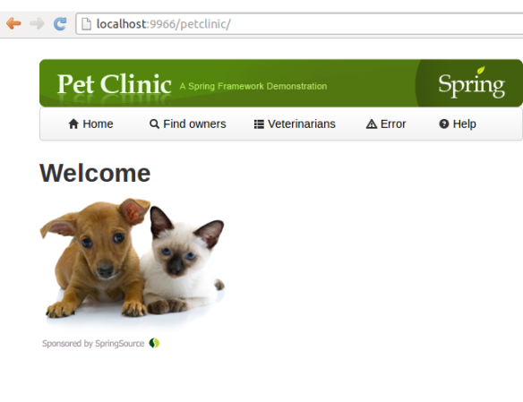
Now we can run the maven command to compile the code, initialize and populate NuoDB tables and then listen to port 9966 for requests.

 $ mvn tomcat7:run

and we can connect Spring using http://localhost:9966/petclinic/.

Spring-PetClinic-1

Spring PetClinic using NuoDB on AWS

Until now we used a local NuoDB instance, it is time to migrate the database layer onto AWS cloud. To run NuoDB on AWS EC2 instances, one of the simplest options is to use AWS CloudFormation. There are CloudFormation templates available on github.

To download them, we can run

$ git clone https://github.com/nuodb/cloudformation.git

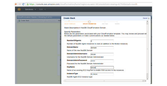
Then we need to open AWS management console, go to CloudFormation and select Create Stack and upload the NuoDB template. (e.g. NuoDB-1.1.template in our case). Then we can define the number of agents (in addition to the broker), the domainname, the domain admin username and password and the EC2 instance type.

NuoDB-CF-1

Once we click on continue, the EC2 instances are going to be created, the status first will be  CREATE_IN_PROGRESS, then CREATE_COMPLETE.

As a result, we will get 3 EC2 instances (since we selected 2 agents); one dedicated to NuoDB broker and the other two for NuoDB agents. We will also have 3 EBS volumes, one for each EC2 instance.

CAUTION: The NuoDB CloudFormation script uses an EC2 auto-scaling group which ensures that the number of agents you selected will always be running. As a result, if you just stop the EC2 instances at the end of your test, AWS will restart them. In order to stop everything properly and clean up your test environment, open the AWS management console, go to CloudFormation, select the NuoDB stack and click “Delete Stack.” This will terminate all instances that were started by the CloudFormation template. More on AWS auto-scaling and how to use the command line tool can be found on AWS website.

Now we can connect to the EC2 host that runs the NuoDB broker:

NuoDB-Console-1

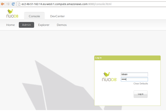
Once we logged in, we can start a database:

NuoDB-Console-2

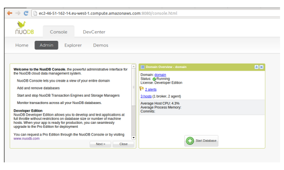
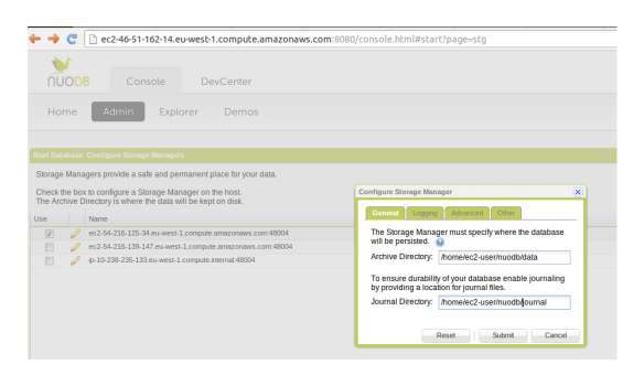
In the next steps we can define the database name (spring), leave “allow non-durable database” option un-selected and the archive and journal directories for storage manager running on one of the hosts (/home/ec2-user/nuodb/data and /home/ec2-user/nuodb/journal respectively). Please, note that the /home/ec2-user directory has to have the appropriate rights to allow the creation of the data and journal directory (e.g. -rwxrwxrwx in our test).

NuoDB-Console-3

After that we can define the transaction engine running on the other EC2 host:

NuoDB-Console-4

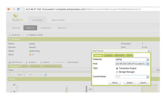
Now we have 3 EC2 hosts : one dedicated to NuoDB broker to serve client connections, one for the storage manager with filesystem storage and one for the transaction engine.

Now, if we change the jdbc connection string in Spring PetClinic (remember, it is defined in data-access.properties), we can connect our application to the NuoDB using AWS servers. The reason why the connection is possible because AWS security groups allow any servers to be connected.

$ vi data-access.properties
#jdbc.url=jdbc:com.nuodb://192.168.80.128/spring?schema=user
jdbc.url=jdbc:com.nuodb://ec2-46-51-162-14.eu-west-1.compute.amazonaws.com/spring?schema=user

We can then rerun the Spring PetClinic command, this time with the database in the AWS cloud:

$ mvn tomcat7:run

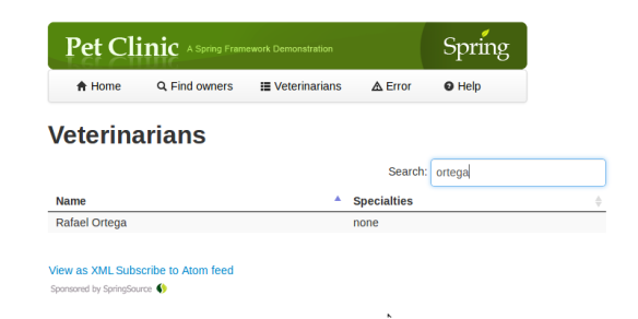
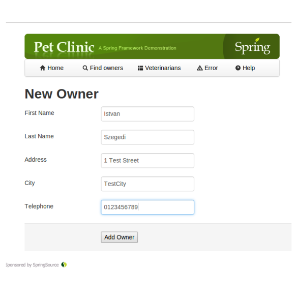
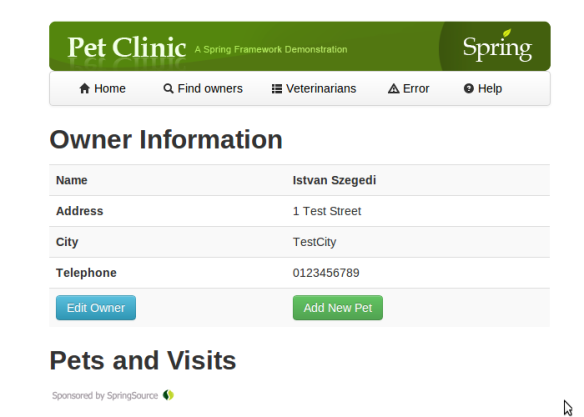
Once Tomcat server is up and running, we can go to http://ec2-46-51-162-14.eu-west-1.compute.amazonaws.com:9966/petclinic/  and  we can search for vets, we can add new owners, we can search for them,  etc.

PetClinic-3

PetClinic-1

PetClinic-2

Scale out and Resilience

Scale out is a method of adding computing resources by adding additional computers to the system, rather than increasing the computing resources on the computers in the system.  Resilience is the ability to provide and maintain an acceptable level of service in case of faults.

If we want to scale out our database and also make it resilient, we can simply go back to the NuoDB console and add a new process using the Add Process menu. For instance, we can add a transaction engine to the EC2 server that was originally running the storage manager, and we can also add a storage manager to the EC2 server previously running a transaction server. This way, we have two EC2 servers both running one instance of the transaction engine and the storage manager.

Scaling out the database is a seamless process for the Spring PetClinic application; we just start up another EC2 server with an agent and add a transaction engine or a storage engine.

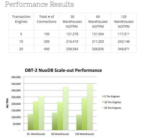
As can be seen in the NuoDB Performance Report, NuoDB scales almost linearly. The diagram below shows how number of transactions per second (TPS) can be increased by adding a new node:

NuoDBPerf

Conclusion

As we have seen in this series, NuoDB combines the standard SQL and ACID properties with elastic scalability that makes it perfectly suitable to be a robust cloud data management system of the 21st century. Its unique architectural approach provides high performance reads and writes and geo-distributed 24/7 operations with built-in resilience. Moreover,applications using well-know frameworks such as Spring and Hibernate can be easily ported or developed with NuoDB as a NewSQL database that meets cloud scale demands.

Large Scale Data Analytics with XtremeData Parallel SQL Database Engine


Introduction

A few months ago I have posted an article about Amazon Web Services Redshift – Amazon’s Data Warehouse solution in the cloud. XtremeData dbX is a similar massive parallel SQL database engine that can be run on-premise as well as in the cloud. It is a purpose-built high-performance and scalable solution for data warehouse applications and large scale analytics using innovative technologies such as vector execution model, dynamic data distribution and automatic load balancing.

XtremeData dbX Architecture

XtremeData dbX is a full SQL and ACID compliant database engine based on shared-nothing, massive parallel query execution. The underlying technology relies on PostgreSQL (similarly to AWS Redshift). In essence, the key architecture components are the head node and multiple data nodes – this is a fairly common patterns in massive parallel execution scenarios.

The head node manages the client connections, parses and plans the queries and sends the result back to the clients. The data nodes manage data storage and execute queries.

dbx-query-exec

XtremeData dbX in AWS cloud

Besides the on-premise deployment option, XtremeData dbX is available in AWS cloud. We need to go to AWS Marketplace to register for it.There are different editions; one for dbX Head and another for dbX Data nodes.

dbx-awsmarketplace

XtremeData provides a document how to setup dbX head and data nodes in the AWS cloud but I decided to implement AWS CloudFormation templates to make the deployment easier. Since there are two different AMIs for head and data nodes, I created two templates.

The AWS CloudFormation dbX-Head template:

{
  "AWSTemplateFormatVersion": "2010-09-09",
  "Description": "XtremeData dbX-Head CloudFormation",
  "Parameters" : {
    "ClusterName" : {
      "Description" : "Name of the XtremeData Cluster",
      "Type" : "String",
      "MinLength": "1",
      "MaxLength": "64",
      "AllowedPattern" : "[-_ a-zA-Z0-9]*",
      "ConstraintDescription" : "can contain only alphanumeric characters, spaces, dashes and underscores."
    },
    "KeyName" : {
      "Description" : "Name of an existing EC2 KeyPair to enable SSH access to the instances",
      "Type" : "String",
      "MinLength": "1",
      "MaxLength": "64",
      "AllowedPattern" : "[-_ a-zA-Z0-9]*",
      "ConstraintDescription" : "can contain only alphanumeric characters, spaces, dashes and underscores."
    },
    "InstanceType" : {
        "Description" : "XtremeData dbX-Head EC2 instance type",
        "Type" : "String",
        "Default" : "m1.medium",
        "AllowedValues" : [ "m1.medium","m1.large","m1.xlarge","m2.xlarge","m2.2xlarge","m2.4xlarge", "c1.xlarge","hi1.4xlarge"],
        "ConstraintDescription" : "must be a valid EC2 instance type."
      }
  },
  "Mappings" : {
    "AWSRegion2AMI" : {
      "us-east-1"      : {"AMI" : "ami-4c2f5d25"},
      "us-west-2"      : {"AMI" : "ami-c127b7f1"},
      "us-west-1"      : {"AMI" : "ami-84cde4c1"}
    }
  },
  "Resources": {
    "XtremeDataSecurityGroup": {
      "Type": "AWS::EC2::SecurityGroup",
      "Properties": {
        "GroupDescription": "Enable XTremedata Access",
        "SecurityGroupIngress": [
          {
            "IpProtocol": "tcp",
            "FromPort": "22",
            "ToPort": "22",
            "CidrIp": "0.0.0.0/0"
          }
        ]
      }
    },
	"XtremeDataSecurityGroupIngress" : {
	   "Type": "AWS::EC2::SecurityGroupIngress",
	   "Properties": {
            "GroupName": { "Ref": "XtremeDataSecurityGroup" },
            "IpProtocol": "tcp",
            "FromPort": "0",
            "ToPort": "65535",
            "SourceSecurityGroupName": { "Ref": "XtremeDataSecurityGroup" }
       }
	},
    "XtremeDataHeadInstance": {
      "Type": "AWS::EC2::Instance",
      "Properties": {
		"UserData" : { "Fn::Base64" : { "Ref" : "ClusterName" }},
        "SecurityGroups": [ { "Ref": "XtremeDataSecurityGroup" } ],
		"ImageId" : { "Fn::FindInMap" : [ "AWSRegion2AMI", { "Ref" : "AWS::Region" }, "AMI" ]},
        "InstanceType": {"Ref" : "InstanceType"},
        "KeyName": { "Ref" : "KeyName" },
		"BlockDeviceMappings" : [
               {
                  "DeviceName" : "/dev/sdf",
                  "Ebs" : {
                     "VolumeType" : "standard",
                     "DeleteOnTermination" : "true",
                     "VolumeSize" : "100"
                  }
               },
               {
                  "DeviceName" : "/dev/sdg",
                  "Ebs" : {
                     "VolumeType" : "standard",
                     "DeleteOnTermination" : "true",
                     "VolumeSize" : "100"
                  }
               },
			   {
                  "DeviceName" : "/dev/sdh",
                  "Ebs" : {
                     "VolumeType" : "standard",
                     "DeleteOnTermination" : "true",
                     "VolumeSize" : "100"
                  }
               },
               {
                  "DeviceName" : "/dev/sdi",
                  "Ebs" : {
                     "VolumeType" : "standard",
                     "DeleteOnTermination" : "true",
                     "VolumeSize" : "100"
                  }
               }
            ],
        "Tags" : [
          { "Key" : "Name", "Value" : "XtremeData dxX-Head"}
        ]
      }
    }
  }
}

This will create the security group for dbX node communications, define userdata (cluster name) and allocate 4 EBS volumes (100 GB each) to dbX Head node.

The AWS CloudFormation dbX-Data template looks as follows:

{
  "AWSTemplateFormatVersion": "2010-09-09",
  "Description": "XtremeData dbX-Data CloudFormation",
  "Parameters" : {
    "ClusterNameAnddbXHead" : {
      "Description" : "Name of the XtremeData Cluster and the dbX-Head EC2 hostname concatenated with semi-colon",
      "Type" : "String",
      "MinLength": "1",
      "MaxLength": "64"
    },
	"XtremeSecurityGroup" : {
      "Description" : "Name of the XtremeData SecurityGroup",
      "Type" : "String",
      "MinLength": "1",
      "MaxLength": "64",
      "AllowedPattern" : "[-_ a-zA-Z0-9]*",
      "ConstraintDescription" : "can contain only alphanumeric characters, spaces, dashes and underscores."
    },
	"NumberOfDataNodes" : {
      "Description" : "Max. Number of Xtreme Data Instances to start (in addition to the Head Instance)",
      "Type" : "Number",
      "Default" : "2"
    },
    "HeadAvailZone" : {
      "Description" : "Name of the Availability Node where dbX-Head instance is running",
      "Type" : "String",
	  "MinLength": "1",
      "MaxLength": "64",
      "AllowedPattern" : "[-_ a-zA-Z0-9]*",
      "ConstraintDescription" : "can contain only alphanumeric characters, spaces, dashes and underscores."
    }, 
    "KeyName" : {
      "Description" : "Name of an existing EC2 KeyPair to enable SSH access to the instances",
      "Type" : "String",
      "MinLength": "1",
      "MaxLength": "64",
      "AllowedPattern" : "[-_ a-zA-Z0-9]*",
      "ConstraintDescription" : "can contain only alphanumeric characters, spaces, dashes and underscores."
    },
    "InstanceType" : {
        "Description" : "XtremeData dbX-Data EC2 instance type",
        "Type" : "String",
        "Default" : "m1.large",
        "AllowedValues" : [ "m1.large","m1.xlarge","m2.xlarge","m2.2xlarge","m2.4xlarge", "c1.xlarge","hi1.4xlarge"],
        "ConstraintDescription" : "must be a valid EC2 instance type."
      }
  },
  "Mappings" : {
    "AWSRegion2AMI" : {
      "us-east-1"      : {"AMI" : "ami-442c5e2d"},
      "us-west-2"      : {"AMI" : "ami-1d28b82d"},
      "us-west-1"      : {"AMI" : "ami-66cce523"}
    }
  },
  "Resources": {
    "XtremeDataNodeGroup" : {
      "Type" : "AWS::AutoScaling::AutoScalingGroup",
      "Properties" : {
        "AvailabilityZones" : [ { "Ref" : "HeadAvailZone" } ],
        "LaunchConfigurationName" : { "Ref" : "DataNodeLaunchConfig" },
        "MinSize" : "0",
        "MaxSize" : {"Ref" : "NumberOfDataNodes"},
		"DesiredCapacity" : {"Ref" : "NumberOfDataNodes"},
        "Tags" : [
          { "Key" : "Name", "Value" : "XtremeData dbX-Data", "PropagateAtLaunch" : "true" }
        ]
      }
    },

	"DataNodeLaunchConfig" : {
       "Type" : "AWS::AutoScaling::LaunchConfiguration",
	   "Properties": {
	      "UserData" : { "Fn::Base64" : { "Ref" : "ClusterNameAnddbXHead" }},
          "KeyName" : { "Ref" : "KeyName" },
          "SecurityGroups" : [ { "Ref" : "XtremeSecurityGroup" } ],
          "InstanceType" : { "Ref" : "InstanceType" },
		  "ImageId" : { "Fn::FindInMap" : [ "AWSRegion2AMI", { "Ref" : "AWS::Region" }, "AMI" ]},
		  "BlockDeviceMappings" : [
               {
                  "DeviceName" : "/dev/sdf",
                  "Ebs" : {
                     "VolumeType" : "standard",
                     "DeleteOnTermination" : "true",
                     "VolumeSize" : "100"
                  }
               },
               {
                  "DeviceName" : "/dev/sdg",
                  "Ebs" : {
                     "VolumeType" : "standard",
                     "DeleteOnTermination" : "true",
                     "VolumeSize" : "100"
                  }
               },
			   {
                  "DeviceName" : "/dev/sdh",
                  "Ebs" : {
                     "VolumeType" : "standard",
                     "DeleteOnTermination" : "true",
                     "VolumeSize" : "100"
                  }
               },
               {
                  "DeviceName" : "/dev/sdi",
                  "Ebs" : {
                     "VolumeType" : "standard",
                     "DeleteOnTermination" : "true",
                     "VolumeSize" : "100"
                  }
               }
          ]
		}
    }
  }
}

This template uses cluster name and AWS EC2 hostname concatenated with ; for userdata, it also uses the availability zones for dbX Head node and the security group that we just defined for dbX Head node. In addition, it allows to define the number of data nodes – it will be used to configure an auto-scaling group to ensure that we have the requested amount of data instances running.

CAUTION: Please, note that it is not enough just to terminate the nodes if you have auto-scaling defined since AWS will initiate new nodes. We need to terminate the instances using as-terminate-instance-in-auto-scaling-group command and then delete the auto-scaling config with as-delete-auto-scaling-group and as-delete-launch-config. More information about AWS auto-scaling can be found here.

To start an XtremeData dbX Head node, we need to go to AWS console Cloud Formation section, then select Create Stack:

dbx-2

Once we submit the configuration, the status will become CREATE_IN_PROGRESS and then after a while CREATE_COMPLETE.

Then we can create another stack for the data nodes using the second CloudFormation template:

dbx-8

After a while we should see one head node and the requested number of datanodes running in AWS EC2 console:

dbx-10

Creating a database in ExtremeData dbX

Once we have fired up the nodes, we can login to the head node as ec2-user using ssh (or e.g. putty on Windows).

First we need to initiate the cluster (please, note that this is a destructive operation, no data will be preserved), then start the cluster and the dbX database engine:

[ec2-user@ip-10-224-122-90 home]$ cluster_init -i 2
init started
examining nodes
initializing head ebs disks: xvdf xvdg xvdh xvdi
mdadm: Defaulting to version 1.2 metadata
mdadm: array /dev/md0 started.
mkfs.xfs: Specified data stripe unit 512 is not the same as the volume stripe unit 128
initializing node ebs disks: xvdf xvdg xvdh xvdi
clearing head ephemeral disks
clearing nodes ephemeral disks
cluster_init done

[ec2-user@ip-10-224-122-90 home]$ cluster_start
initializing head ephemeral disks
  head ephemeral disks:  xvdb
    raid-ing
mdadm: /dev/xvdb appears to contain an ext2fs file system
    size=419395584K  mtime=Sat Jul  6 21:52:00 2013
mdadm: Defaulting to version 1.2 metadata
mdadm: array /dev/md1 started.
mkfs.xfs: Specified data stripe unit 512 is not the same as the volume stripe unit 128
mkfs.xfs: Specified data stripe width 512 is not the same as the volume stripe width 128
examining nodes
assembling node EBSs: xvdf xvdg xvdh xvdi
initializing node tmp disks: xvdb xvdc
  raid-ing
cluster_start done

[ec2-user@ip-10-224-122-90 home]$ dbx_start
new dbx installation initialized
Initializing kernel nfsd:                                  [  OK  ]
Starting NFS services:                                     [  OK  ]
Starting NFS mountd:                                       [  OK  ]
Stopping RPC idmapd:                                       [  OK  ]
Starting RPC idmapd:                                       [  OK  ]
Starting NFS daemon:                                       [  OK  ]
rpc.svcgssd is stopped
rpc.mountd (pid 3402) is running...
nfsd (pid 3467 3466 3465 3464 3463 3462 3461 3460) is running...
Generating binary repository file ...
file 'xdapp.conf2.txt.conf0' generated.
starting dbx nodes
Starting xdu daemon...                                     [  OK  ]
dbx startup done
[ec2-user@ip-10-224-122-90 home]$
[ec2-user@ip-10-224-122-90 home]$

Now we can login as dbxdba user (we can do it again with ssh or putty since the key is copied over from ec2-user). Then we need to change the dbxdba password (using passwd Linux commad) in order to be able to login using dbX tools.

Now we are ready to create a server and once the server is created, we can then create a database. The simplest way to manage the database and run SQL queries is to use a command line tool called xdudb:

$ xdudb create aws_server 32145
||==================||

[dbxdba@ip-10-224-122-90 ~]$ xdudb list
||==================||
aws_server
[dbxdba@ip-10-224-122-90 ~]$ xdudb status
||==================||
ip-10-224-122-90 configuration: 1 head node and 2 data nodes
running dbx services          : 1 head node and 2 data nodes

[dbxdba@ip-10-224-122-90 ~]$ xdudb start aws_server
||==================||

[dbxdba@ip-10-224-122-90 ~]$ xdudb info aws_server
||==================||
Name        : aws_server
NodeSet     : Default_NS
Owner       : dbxdba
Port        : 32145
H|0   |head    |10.224.122.90  |head |/volumes/data/dbstore/dbxdba/aws_server/head
D|1   |node00  |10.154.137.31  |n0   |/hd/dbxdba/aws_server/n0
D|2   |node01  |10.165.7.225   |n1   |/hd/dbxdba/aws_server/n1

[dbxdba@ip-10-224-122-90 ~]$ xdudb dbcreate aws_server aws_db
CREATE DATABASE

Now we can create a table, insert some rows and run select statements.

[dbxdba@ip-10-224-122-90 ~]$ xdudb sql aws_server aws_db
Welcome to dbX psql 3.2.5, the interactive SQL terminal.

Type:  \copyright for distribution terms
       \h for help with SQL commands
       \? for help with psql commands
       \g or terminate with semicolon to execute query
       \q to quit

aws_db=# CREATE TABLE products (
aws_db(# product_no INTEGER,
aws_db(# name VARCHAR(30),
aws_db(# price NUMERIC(10,2)
aws_db(# );
CREATE TABLE
aws_db=# INSERT INTO products VALUES(1, 'Product1', 100.00);
INSERT 0 1
aws_db=# SELECT * FROM products;
 product_no |   name   | price
------------+----------+--------
          1 | Product1 | 100.00
(1 row, Query Total: 1)

WIth the help of the xdudb command line tool we can check dbX version, check disk usage and mounted filesystems, etc.

[dbxdba@ip-10-224-122-90 ~]$ xdudb version
ip-10-224-122-90        2013-07-07 00:03:10
  DB           : dbX SQL 3.2.5
               : fpga.run r4347
  command line : xdudb 1.4
  GUI          : xdadm 3.0.2
  daemon       : xdutils 4.5.8
  OS           : Linux 3.4.43-43.43.amzn1.x86_64

[dbxdba@ip-10-224-122-90 ~]$ xdudb  du aws_server
||==================||
H|0   |head    |10.224.122.90  |head |60M  |/volumes/data/dbstore/dbxdba/aws_server/head
D|1   |node00  |10.154.137.31  |n0   |58M  |/hd/dbxdba/aws_server/n0
D|2   |node01  |10.165.7.225   |n1   |58M  |/hd/dbxdba/aws

[dbxdba@ip-10-224-122-90 ~]$ xdudb  df
head : 10.224.122.90
Filesystem            Size  Used Avail Use% Mounted on
/dev/md0              400G   95M  400G   1% /volumes/data
node00 : 10.154.137.31
Filesystem            Size  Used Avail Use% Mounted on
/dev/md0              400G   93M  400G   1% /volumes/data
node01 : 10.165.7.225
Filesystem            Size  Used Avail Use% Mounted on
/dev/md0              400G   93M  400G   1% /volumes/data

xdAdm web based management GUI

In addition to the command line tool that we described in the AWS cloud deployment scenario, there is also a web base GUI to manage the applicance – it is based on Apache Tomcat. We just go to http://dbx-headnode:8080/xdadm url and login. The we can manage the servers and databases, check nodesets and monitor the system:

dbx-15

XtremeData dbX virtual machine

If someone just wants to try out dbX database engine then she can download a virtual machine from XtremeData web site. The instance can be run e.g using vmplayer. Once the user logged in to the virtual machine as dbxdba, he can startup a server:

$ xdudb start dbxtest

Splunk Storm – Machine Data Processing in the Cloud


Introduction

Splunk is a platform to process machine data from various sources such as weblogs, syslogs, log4j logs and can also work with JSON and CSV file formats thus any application that produces JSON or CSV output can be seen as a source for Splunk. As the volume and variety of machine data are increasing, Splunk is becoming a more and more interesting player in big data world, too.

Splunk can be considered as a search engine for IT data. Splunk collects data from multiple sources, indexes them and the users can search them using Splunk proprietary language called SPL (Search Processing Language). The search results can then be used to create reports and dashboards to visualize the data.

Splunk Architecture

Under the hood Splunk architecture has the following key components:
forwarders are used to forward data to Splunk receiver instances. Receiver instances are normally indexers.
indexers that are splunk instances to index data. Indexes are stored in files. There are two types of files; raw datafiles which store the data in compressed format and index files that contain metadata for search queries. During indexing, Splunk extracts default fields and identifies events based on timestamps or creates them if there is no timestamp found.
search head and search peers. In a distributed environment search head manages the search requests, directs them to search peers and then merges result back to the users.
Splunk Web is a graphical user interface based on Python application server.
SplunkArchitecture

Splunk Storm

Splunk Storm is a cloud service version of Splunk. Splunk Storm runs in the Amazon cloud and uses of both Elastic Block Storage (EBS) and the Simple Storage Service (S3).

The price plan is based on monthly fee, it depends on the volume of the data that you want to store. As of writing this article, there is a free tier with 1 GB storage, while for example 100 GB storage volume costs 400 USD and the maximum 1 TB storage volume costs 3,000 USD per month.

To get started, we need to sign up and crate a project.
Splunk-1

Then we can define the data inputs. There are four options: upload a file, use forwarders, use the API (it is in beta yet) or use network data sent directly from the servers.

As a first test, we will use data files uploaded from a local directory. We used a sample apache web access.log and a syslog available from http://www.monitorware.com/en/logsamples/

It takes a some time to index the files and then they become available for search queries.

Splunk-11

We can run a search query to identify all HTTP client side error codes:

"source="access_log.txt" status>="400" AND status <="500"

Splunk-15

If we want to identify all the access log entries with HTTP POST method, we can run the following search query:

source="access_log.txt" method="POST"

In a similar way, if we want to find all the messages from the uploaded syslog file that were generated by the kernel process then we can run the following query:

source="syslog-messages.txt" process="kernel"

Splunk-16

Splunk forwarder and Twitter API

As a next example, we want to test output generated by our program using Twitter API. The program will generate JSON format in a file using Python based Twitter API. The directory is monitored by a Splunk forwarder and once the file is created in the predefined directory, the forwarder will send it to Splunk Storm.

First we need to create an application in Twitter via https://dev/twitter.com portal. The application will have its customer_key, customer_secret, access_token_key and access_token_secret that is going to be required by the Twitter API.

Twitter-6

The Twitter API that we are going to use for the Python application is downloadable from Github, https://github.com/bear/python-twitter.git .

This API depends oauth2, simplejson and httplib2 so we need to installed them first. Then we can get the code from Github and build and install the package.

$ git clone https://github.com/bear/python-twitter.git

# Build and Install:
$ python setup.py build
$ python setup.py install

The Twitter application code – twtr.py –  is as follows:

# twtr.py
import sys
import twitter

if len(sys.argv) < 3:
    print "Usage: " + sys.argv[0] + " keyword count"
    sys.exit(1)

keyword = sys.argv[1]
count = sys.argv[2]
# Twitter API 1.1. Count - up to a maximum of 100
# https://dev.twitter.com/docs/api/1.1/get/search/tweets
if int(count) > 100:
    count = 100

api = twitter.Api(consumer_key="CONSUMER_KEY", consumer_secret="CONSUMER_SECRET", access_token_key="ACCESS_TOKEN_KEY", access_token_secret="4PXvz7QIiwtwhFrFXFEkc9wY7iBOdgusD8ZQLvUhabM" )

search_result = api.GetSearch(term=keyword, count=count)

for s in search_result:
    print s.AsJsonString()

The Python program can be run as follows:

$ python twtr.py "big data" 100

Installing Splunk forwarder

Then we need to install Splunk forwarder, see http://www.splunk.com/download/universalforwarder . We also need to download the Splunk credentials that will allow the forwarder to send data to our project. Once the forwarder and the ceredentials are installed we can login and add a directory (twitter_status) for our forwarder to be monitored. We defined the sourcetype as json_notimestamp.

# Download splunk forwarder
$ wget -O splunkforwarder-5.0.3-163460-Linux-x86_64.tgz 'http://www.splunk.com/page/download_track?file=5.0.3/universalforwarder/linux/splunkforwarder-5.0.3-163460-Linux-x86_64.tgz&ac=&wget=true&name=wget&typed=releases&elq=8ccba442-db76-4fc8-b36b-36252bb61257'

# Install and start splunk forwarder
$ tar xvzf splunkforwarder-5.0.3-163460-Linux-x86_64.tgz
$ export SPLUNK_HOME=/home/ec2-user/splunkforwarder
$ $SPLUNK_HOME/bin/splunk start
# Install project credentials
$ $SPLUNK_HOME/bin/splunk install app ./stormforwarder_2628fbc8d76811e2b09622000a1cdcf0.spl -auth admin:changeme
App '/home/ec2-user/stormforwarder_2628fbc8d76811e2b09622000a1cdcf0.spl' installed

# Login
$SPLUNK_HOME/bin/splunk login -auth admin:changeme

#' Add monitor (directory or file)
 $SPLUNK_HOME/bin/splunk add monitor /home/ec2-user/splunk_blog/twitter_status -sourcetype json_no_timestamp
Added monitor of '/home/ec2-user/splunk_blog/twitter_status'.

Now we are ready to run the Python code using Twitter API:

$ python twtr.py "big data" 100 | tee twitter_status/twitter_status.txt

The program creates a twitter_status.txt file under twitter_status directory which is monitored by Splunk forwarder. The forwarder sends the output file to Splunk Storm. After some time it will appears under the inputs sections as authenticated forwarder. The  file will be shown as a source together with the previously uploaded apache access log and syslog.
SPlunk-17

Splunk-18

If we want to search for users with location London, the search query looks like this:

source="/home/ec2-user/splunk_blog/twitter_status/twitter_status.txt" user.location="London, UK"

We can also define a search query to show the top 10 timezones from the Twitter result and from the search result it is easy to create a Report with just a few clicks on the web user interface. The report allows to chose multiple visualization options like column, area or pie chart types, etc.

source="/home/ec2-user/splunk_blog/twitter_status/twitter_status.txt" | top limit=10 user.time_zone

SPlunk-22

Splunk-25

Conclusion

As mentioned in the beginning of this article, the variety and the volume generated by machines are increasing dramatically; sensor data, application logs, web access logs, syslogs, database and filesystem audit logs are just a few examples of the potential data sources that require attention but can pose difficulties to process and analyse them in a timely manner. Splunk is a great tool to deal with the ever increasing data volume and with Splunk Storm users can start analysing their data in the cloud without hassle.