Apache Phoenix – an SQL Driver for HBase


Introduction

HBase is one of the most popular NoSQL databases, it is available in all major Hadoop distributions and also part of AWS Elastic MapReduce as an additional application. Out of the box it has its own data model operations such as Get, Put, Scan and Delete and it does not offer SQL-like capabilities, as oppose to, for instance, Cassandra query language, CQL.
Apache Phoenix is a SQL layer on top of HBase to support the most common SQL-like operations such as CREATE TABLE, SELECT, UPSERT, DELETE, etc. Originally it was developed by Salesforce.com engineers for internal use and was open sourced. In 2013 it became an Apache incubator project.

Architecture

We have covered HBase in more detail in this article. Just a quick recap: HBase architecture is based on three key components: HBase Master server, HBase Region Servers and Zookeeper.

HBase-Architecture

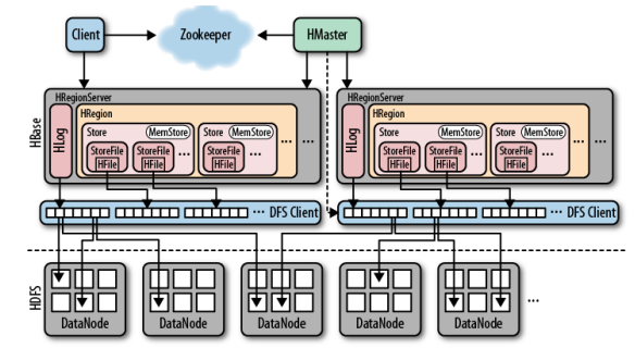
The client needs to find the RegionServers in order to work with the data stored in HBase. In essence, regions are the basic elements for distributing tables across the cluster. In order to find the Region servers, the client first will have to talk to Zookeeper.

HBase-Lookup

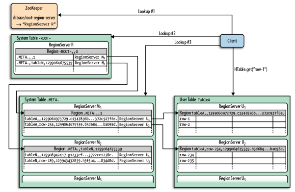
The key elements in the HBase datamodel are tables, column families, columns and rowkeys. The tables are made of columns and rows. The individual elements at the column and row intersections (cells in HBase term) are version based on timestamp. The rows are identified by rowkeys which are sorted – these rowkeys can be considered as primary keys and all the data in the table can be accessed via them.

The columns are grouped into column families; at table creation time you do not have to specify all the columns, only the column families. Columns have a prefix derived from the column family and its own qualifier,a column name looks like this: ‘contents:html’.

As we have seen, HBase classic data model is not designed with SQL in mind. Under the hood it is a sorted multidimensional Map. That is where Phoenix comes to the rescue; it offers a SQL skin on HBase. Phoenix is implemented as a JDBC driver. From architecture perspective a Java client using JDBC can be configured to work with Phoenix Driver and can connect to HBase using SQL-like statements. We will demonstrate how to use SQuirreL client, a popular Java-based graphical SQL client together with Phoenix.

Getting Started with Phoenix

You can download Phoenix from Apache download site. Different Phoenix versions are compatible with different HBase versions, so please, read Phoenix documentation to ensure you have the correct setup. In our tests we used Phoenix 3.0.0 with HBase 0.94, the Hadoop distribution was Cloudera CDH4.4 with Hadoop v1.. The Phoenix package contains both Hadoop version 1 and version 2 drivers for the clients so we had to use the appropriate Hadoop-1 files, see the details later on when talking about SQuirreL client.

Once you unzipped the downloaded Phoenix package, you need to copy the relevant Phoenix jar files to the HBase region servers in order to ensure that the Phoenix client can communicate with them, otherwise you may get an error message saying that the client and server jars are not compatible.

$ cd ~/phoenix/phoenix-3.0.0-incubating/common
$ cp phoenix-3.0.0-incubating-client-minimal.jar  /usr/lib/hbase/lib
$ cp phoenix-core-3.0.0-incubating.jar /usr/lib/hbase/lib

After you copied the jar files to the region servers, we had to restart them.

Phoenix provides a command line tool called sqlline – it is a utility written in Python. Its functionality is similar to Oracle SQLPlus or MySQL command line tools; not too sophisticated but does the job for simply use cases.

Before you start using sqlline, you can create a sample database table, populate it and run some simple queries as follows:

$ cd ~/phoenix/phoenix-3.0.0.0-incubating/bin
$ ./psql.py localhost ../examples/web_stat.sql ../examples/web_stat.csv ../examples/web_stat_queries.sql

This will run a CREATE TABLE statement:

CREATE TABLE IF NOT EXISTS WEB_STAT (
     HOST CHAR(2) NOT NULL,
     DOMAIN VARCHAR NOT NULL,
     FEATURE VARCHAR NOT NULL,
     DATE DATE NOT NULL,
     USAGE.CORE BIGINT,
     USAGE.DB BIGINT,
     STATS.ACTIVE_VISITOR INTEGER
     CONSTRAINT PK PRIMARY KEY (HOST, DOMAIN, FEATURE, DATE)
);

Then load the data stored in the web_stat CSV file:

NA,Salesforce.com,Login,2013-01-01 01:01:01,35,42,10
EU,Salesforce.com,Reports,2013-01-02 12:02:01,25,11,2
EU,Salesforce.com,Reports,2013-01-02 14:32:01,125,131,42
NA,Apple.com,Login,2013-01-01 01:01:01,35,22,40
NA,Salesforce.com,Dashboard,2013-01-03 11:01:01,88,66,44
...

And the run a few sample queries on the table, e.g.:

-- Average CPU and DB usage by Domain
SELECT DOMAIN, AVG(CORE) Average_CPU_Usage, AVG(DB) Average_DB_Usage 
FROM WEB_STAT 
GROUP BY DOMAIN 
ORDER BY DOMAIN DESC;

Now you can connect to HBase using sqlline:

$ ./sqlline.py localhost
[cloudera@localhost bin]$ ./sqlline.py localhost
..
Connecting to jdbc:phoenix:localhost
Driver: org.apache.phoenix.jdbc.PhoenixDriver (version 3.0)
Autocommit status: true
Transaction isolation: TRANSACTION_READ_COMMITTED
..
Done
sqlline version 1.1.2
0: jdbc:phoenix:localhost> select count(*) from web_stat;
+------------+
|  COUNT(1)  |
+------------+
| 39         |
+------------+
1 row selected (0.112 seconds)
0: jdbc:phoenix:localhost> select host, sum(active_visitor) from web_stat group by host;
+------+---------------------------+
| HOST | SUM(STATS.ACTIVE_VISITOR) |
+------+---------------------------+
| EU   | 698                       |
| NA   | 1639                      |
+------+---------------------------+
2 rows selected (0.294 seconds)
0: jdbc:phoenix:localhost>

Using SQuirreL with Phoenix

If you prefer to use a graphical SQL client with Phoenix, you can download e.g. SQuirreL from here. After that the first step is to copy the appropriate Phoenix driver jar file to SQuirreL lib directory:

$ cd ~/phoenix
$ cp phoenix-3.0.0-incubating/hadoop-1/phoenix-3.0.0.-incubatibg-client.jar ~/squirrel/lib

Now you are ready to configure the JDBC driver in SQuirreL client, as shown in the picture below:

Squirrel-1

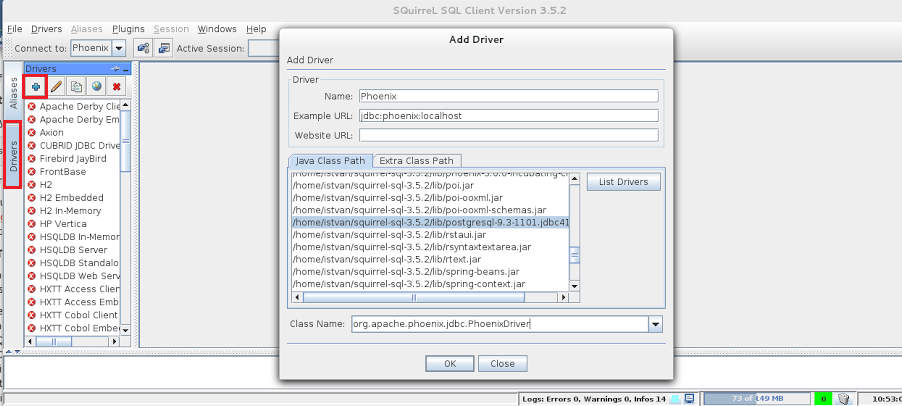
Then you can connect to Phoenix using the appropriate connect string (jdbc:phoenix:localhost in our test scenario):

Squirrel-2

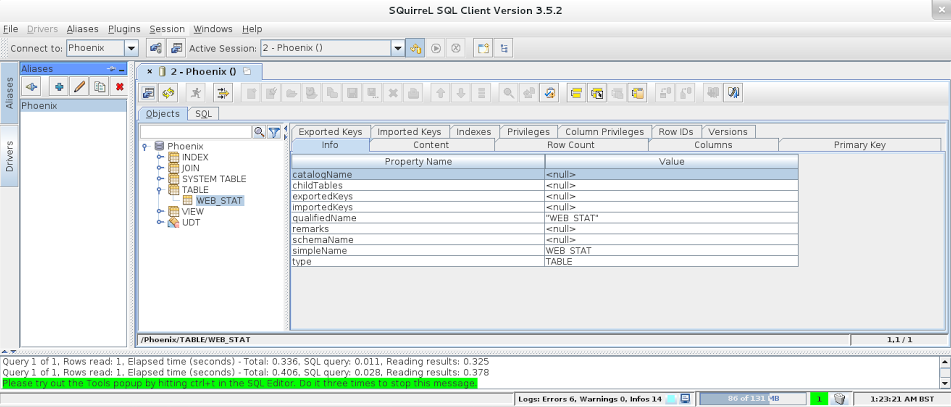
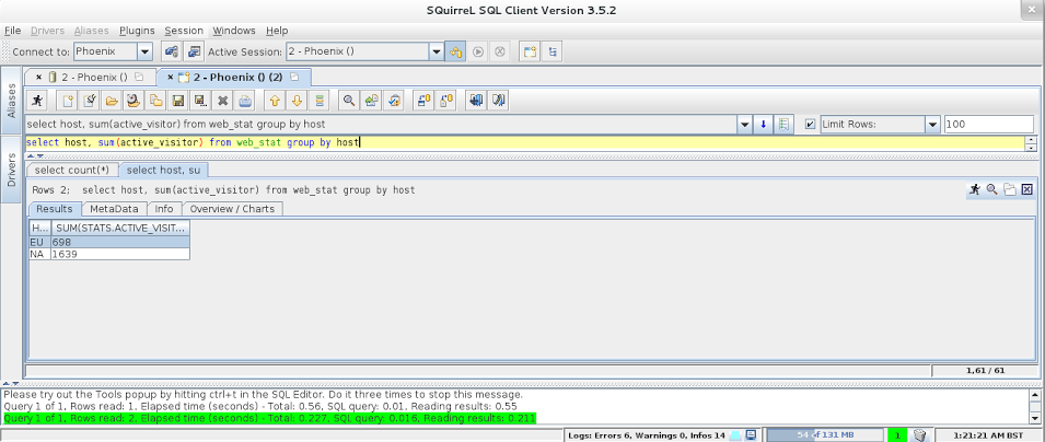
Once connected, you can start executing your SQL queries:
Squirrel-3

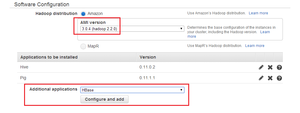
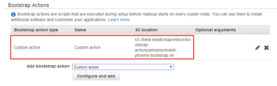
Phoenix on Amazon Web Services – AWS Elastic MapReduce with Phoenix

You can also use Phoenix with AWS Elastic MapReduce. When you create a cluster, you need to specify Apach Hadoop version, then configure HBase as additional application and define the bootsrap action to load Phoenix onto your AWS EMR cluster. See the details below in the pictures:

AWS-EMR-3

AWS-EMR-5

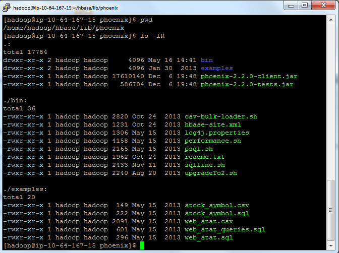
Once the cluster is running, you can login to the master node using ssh and check your Phoenix configuration.
AWS-EMR-9

Conclusion

SQL is one of the most popular languages used by data scientists and it is likely to remain so. With the advent of Big Data and NoSQL databases the volume, variety and velocity of the data have significantly increased but still the demand for traditional, well-known languages to process them did not change too much. SQL on Hadoop solutions are gaining momentum. Apache Phoenix is interesting open source player to offer SQL layer on top of HBase.

Pivotal Hadoop Distribution and HAWQ realtime query engine


Introduction

SQL on Hadoop and the support for interactive, ad-hoc queries in Hadoop is in increasing demand and all the vendors are providing their answer to these requirements. In the open source world Cloudera’s Impala, Apache Drill (backed by MapR), Hortonworks’s Stinger initiatives are competing in this market, just to mention a few key players. There are also strong offerings from BI and analytics vendors such as Pivotal (HAWQ), Teradata (SQL-H) or IBM (BigSQL).
In this post we will cover Pivotal Hadoop Distribution (Pivotal HD) and HAWQ, Pivotal’s interactive distributed SQL query engine.

Getting started with Pivotal HD

Pivotal HD contains the most well-known open source components such as HDFS, MapReduce, YARN, Hive, Pig, HBase, Flume, Sqoop and Mahout. There are also additional components available such as the Command Center, Unified Storage Services, Data Loader, Spring and HAWQ as an add-on. (Pivotal has an offering called GemFire XD which is a distributed in-memory data grid but that is out of scope for our current discussion).

PivotalHD_ArchitectDiagram

Let us take an example how to use Pivotal HD to answer the following question: what was the highest price of the Apple, Google and Nokia stocks ever and when those stocks reached the peak value?

First we are going to develop a MapReduce algorithm to calculate these values and then we will run SQL queries in HAWQ to get the same result. Our test environment is based on Pivotal HD Single Node virtual machine running on VMWare VMPlayer and it is using a 64-bit CentOS 6.4 distribution. Pivotal HD virtual machine does not contain Eclipse so we had to download that separately from eclipse.org.

Once we have the environment set, the next step is to create a maven project.

$ mvn archetype:generate -DarchetypeGroupId=org.apache.maven.archetypes -DarchetypeArtifactId=maven-archetype-quickstart -DgroupId=highest_stock_price -DartifactId=highest_stock_price

This command will create a pom.xml where we have the basic project settings and junit added as a dependency. Then we need to edit pom.xml and add the other relevant dependencies and build settings.
After that we can start writing our Hadoop application in Eclipse. The code is also uploaded to Github (https://github.com/iszegedi/Pivotal-HD-and-HAWQ-blog) for your reference.

pivotal-eclipse-dev

The key Java classes are HighestStockPriceDriver.java which is the main driver file for our MapReduce application, the HighestStockPriceMapper.java which contains the map() function and the HighestStockPriceReducer.java which is running the reduce() function.

Then we can compile the code and package it into a jar file:

$ mvn clean compile
$ mvn -DskipTests package

The next step is to copy our data sets into a Hadoop HDFS directory.

$ hadoop fs -mkdir /stock_demo/input
$ hadoop fs -put *.csv /stock_demo/input/
$ hadoop fs -ls /stock_demo/input/
Found 3 items
-rw-r--r--   1 gpadmin hadoop     403395 2013-12-31 00:25 /stock_demo/input/apple.csv
-rw-r--r--   1 gpadmin hadoop     134696 2013-12-31 00:25 /stock_demo/input/google.csv
-rw-r--r--   1 gpadmin hadoop     248405 2013-12-31 00:25 /stock_demo/input/nokia.csv

The format of the files (apple.csv, nokia.csv, google.csv) is as follows (the columns are Symbol, Date, Open, High, Low, Close, Volume, Adj Close):

$ head -5 apple.csv
AAPL,2013-09-06,498.44,499.38,489.95,498.22,12788700,498.22
AAPL,2013-09-05,500.25,500.68,493.64,495.27,8402100,495.27
AAPL,2013-09-04,499.56,502.24,496.28,498.69,12299300,498.69
AAPL,2013-09-03,493.10,500.60,487.35,488.58,11854600,488.58
AAPL,2013-08-30,492.00,492.95,486.50,487.22,9724900,487.22

Now we are ready to run our MapReduce algorithm on the data sets:

$ hadoop jar target/highest_stock_price-1.0.jar highest_stock_price/HighestStockPriceDriver /stock_demo/input/ /stock_demo/output/

$ hadoop fs -cat /stock_demo/output/part*
AAPL:	2012-09-19	685.76
GOOG:	2013-07-15	924.69
NOK:	2000-06-19	42.24

We can check the status of the Hadoop job using the following command:

$ hadoop job -status job_1388420266428_0001
DEPRECATED: Use of this script to execute mapred command is deprecated.
Instead use the mapred command for it.

13/12/31 00:31:15 INFO service.AbstractService: Service:org.apache.hadoop.yarn.client.YarnClientImpl is inited.
13/12/31 00:31:15 INFO service.AbstractService: Service:org.apache.hadoop.yarn.client.YarnClientImpl is started.
13/12/31 00:31:17 INFO mapred.ClientServiceDelegate: Application state is completed. FinalApplicationStatus=SUCCEEDED. Redirecting to job history server

Job: job_1388420266428_0001
Job File: hdfs://pivhdsne:8020/user/history/done/2013/12/31/000000/job_1388420266428_0001_conf.xml
Job Tracking URL : http://localhost:19888/jobhistory/job/job_1388420266428_0001
Uber job : false
Number of maps: 3
Number of reduces: 1
map() completion: 1.0
reduce() completion: 1.0
Job state: SUCCEEDED
....
....

This will show us that there were 3 mappers and 1 reducer run. It will also show the number of input and output records and bytes.

HAWQ interactive distributed query engine

The common complaints with regards to the classic Hadoop MapReduce algorithms are that they require fairly extensive Java experience and they are rather tuned for batch type of data processing, they are not really suitable for exploratory data analysis using ad-hoc interactive queries. That is where HAWQ can come to the rescue.

HAWQ is a massively parallel SQL query engine. The underlying engine is based on PostgreSQL (version 8.2.15, as of writing this post) so it can support the standard SQL statements out of the box. The key architecture components are HAWQ master, HAWQ segments, HAWQ storage and HAWQ interconnect.

HAWQ-architecture

HAWQ master is responsible for accepting the connections from the clients and it also manages the system tables containing metadata about HAWQ itself (however, no user data is stored on the master). The master then parses and optimises the queries and develops an execution plan which is then dispatched to the segments.

HAWQ segments are the processing units, they are responsible of executing the local database operations on their own data sets.

HAWQ-query-execution

HAWQ stores all the user data in HDFS. HAWQ interconnect refers to the UDP based inter-process communication between the segments.

Now let us see how we can answer the same question about stock prices that we did with our MapReduce job.

First we need to login to our client (psql which is the same client that we know well from PostgeSQL databases) and create our schema and table:

$ psql
psql (8.2.15)
Type "help" for help.

gpadmin=# create schema stock_demo;
gpadmin=# create table stock_demo.stock
gpadmin-# (
gpadmin(# symbol TEXT,
gpadmin(# date TEXT,
gpadmin(# open NUMERIC(6,2),
gpadmin(# high NUMERIC(6,2),
gpadmin(# low NUMERIC(6,2),
gpadmin(# close NUMERIC(6,2),
gpadmin(# volume INTEGER,
gpadmin(# adjclose NUMERIC(6,2)
gpadmin(# )
gpadmin-# with (appendonly=true) distributed randomly;

The next step is to load the data into this HAWQ table, we can use the following commands to do this:

$ cat google.csv | psql -c "COPY stock_demo.stock FROM STDIN DELIMITER E'\,' NULL E'';"
$ cat nokia.csv | psql -c "COPY stock_demo.stock FROM STDIN DELIMITER E'\,' NULL E'';"
$ cat apple.csv | psql -c "COPY stock_demo.stock FROM STDIN DELIMITER E'\,' NULL E'';"

Now we can login again to our psql client and run the SQL queries:

gpadmin=# select count(*) from stock_demo.stock;
 count 
-------
 14296
(1 row)

gpadmin=# select symbol, date, adjclose from stock_demo.stock where adjclose in
gpadmin-# ( select max(adjclose) as max_adj_close from stock_demo.stock 
gpadmin(#   group by symbol )
gpadmin-# order by symbol;
 symbol |    date    | adjclose 
--------+------------+----------
 AAPL   | 2012-09-19 |   685.76
 GOOG   | 2013-07-15 |   924.69
 NOK    | 2000-06-19 |    42.24
(3 rows)

These SQL queries relied on HAWQ internal table,thus we had to load the data into it from our local file system. HAWQ also support the notion of external tables using PXF (Pivotal eXtension Framework). It is an external table interface in HAWQ that allows to read data directly from HDFS directories. It has a concept of fragmenters, accessors and resolvers which are used to split the data files into smaller chunks and read them into HAWQ without having the need to explicitly load them into HAWQ internal tables.

If we want to use external table, we need to create it using the following SQL statement:

gpadmin=# create external table stock_demo.stock_pxf
gpadmin-# (
gpadmin(# symbol TEXT,
gpadmin(# date TEXT,
gpadmin(# open NUMERIC(6,2),
gpadmin(# high NUMERIC(6,2),
gpadmin(# low NUMERIC(6,2),
gpadmin(# close NUMERIC(6,2),
gpadmin(# volume INTEGER,
gpadmin(# adjclose NUMERIC(6,2)
gpadmin(# )
gpadmin-# location ('pxf://pivhdsne:50070/stock_demo/input/*.csv?Fragmenter=HdfsDataFragmenter&Accessor=TextFileAccessor&Resolver=TextResolver')
gpadmin-# format 'TEXT' (delimiter = E'\,');

Then we can run the same queries against the external table as before:

gpadmin=# select count(*) from stock_demo.stock_pxf;
 count 
-------
 14296
(1 row)

gpadmin=# select symbol, date, adjclose from stock_demo.stock_pxf where adjclose in 
gpadmin-# ( select max(adjclose) as max_adj_close from stock_demo.stock_pxf
gpadmin(#   group by symbol )
gpadmin-# order by symbol;
 symbol |    date    | adjclose 
--------+------------+----------
 AAPL   | 2012-09-19 |   685.76
 GOOG   | 2013-07-15 |   924.69
 NOK    | 2000-06-19 |    42.24
(3 rows)

Conclusion

SQL on Hadoop is gaining significant momentum, the demand to be able to run ad-hoc, interactive queries as well as batch data processing on top of Hadoop is increasing. Most of the key players in big data world have started providing solutions to address these needs. 2014 seems to be an interesting year to see how these offerings are going to evolve.