Hadoop REST API – WebHDFS


Introduction

Hadoop provides a Java native API to support file system operations such as create, rename or delete files and directories, open, read or write files, set permissions, etc. A very basic example can be found on Apache wiki about how to read and write files from Hadoop.

This is great for applications running within the Hadoop cluster but there may be use cases where an external application needs to manipulate HDFS like it needs to create directories and write files to that directory or read the content of a file stored on HDFS. Hortonworks developed an additional API to support these requirements based on standard REST functionalities.

WebHDFS REST API

WebHDFS concept is based on HTTP operations like GET, PUT, POST and DELETE. Operations like OPEN, GETFILESTATUS, LISTSTATUS are using HTTP GET, others like CREATE, MKDIRS, RENAME, SETPERMISSIONS are relying on HTTP PUT. APPEND operations is based on HTTP POST, while DELETE is using HTTP DELETE.

Authentication can be based on user.name query parameter (as part of the HTTP query string) or if security is turned on then it relies on Kerberos.

The standard URL format is as follows: http://host:port/webhdfs/v1/?op=operation&user.name=username

In some cases namenode returns a URL using HTTP 307 Temporary Redirect mechanism with a location URL referring to the appropriate datanode. Then the client needs to follow that URL to execute the file operations on that particular datanode.

By default the namenode and datanode ports are 50070 and 50075, respectively, see more details about the default HDFS ports on Cloudera blog.

In order to configure WebHDFS, we need to hdfs-site.xml as follows:

        <property>
           <name>dfs.webhdfs.enabled</name>
           <value>true</value>
        </property>

WebHDFS examples

As the simplest approach, we can use curl to invoke WebHDFS REST API

1./ Check directory status

$ curl -i "http://localhost:50070/webhdfs/v1/tmp?user.name=istvan&op=GETFILESTATUS"
HTTP/1.1 200 OK
Content-Type: application/json
Expires: Thu, 01-Jan-1970 00:00:00 GMT
Set-Cookie: hadoop.auth="u=istvan&p=istvan&t=simple&e=1370210454798&s=zKjRgOMQ1Q3NB1kXqHJ6GPa6TlY=";Path=/
Transfer-Encoding: chunked
Server: Jetty(6.1.26)

{"FileStatus":{"accessTime":0,"blockSize":0,"group":"supergroup","length":0,"modificationTime":1370174432465,"owner":"istvan","pathSuffix":"","permission":"755","replication":0,"type":"DIRECTORY"}}

This is similar to execute the Hadoop ls filesystem command:

$ bin/hadoop fs -ls /
Warning: $HADOOP_HOME is deprecated.

Found 1 items
drwxr-xr-x - istvan supergroup 0 2013-06-02 13:00 /tmp

2./ Create a directory

$ curl -i -X PUT "http://localhost:50070/webhdfs/v1/tmp/webhdfs?user.name=istvan&op=MKDIRS"
HTTP/1.1 200 OK
Content-Type: application/json
Expires: Thu, 01-Jan-1970 00:00:00 GMT
Set-Cookie: hadoop.auth="u=istvan&p=istvan&t=simple&e=1370210530831&s=YGwbkw0xRVpEAgbZpX7wlo56RMI=";Path=/
Transfer-Encoding: chunked
Server: Jetty(6.1.26)

The equivalent Hadoop filesystem command is as follows:

$ bin/hadoop fs -ls /tmp
Warning: $HADOOP_HOME is deprecated.

Found 2 items
drwxr-xr-x   - istvan supergroup          0 2013-06-02 12:17 /tmp/hadoop-istvan
drwxr-xr-x   - istvan supergroup          0 2013-06-02 13:02 /tmp/webhdfs

3./ Create a file

To create a file requires two steps. First we need to run the command against the namenode then follows the redirection and execute the WebHDFS API against the appropriate datanode.

Step 1:

curl -i -X PUT "http://localhost:50070/webhdfs/v1/tmp/webhdfs/webhdfs-test.txt?user.name=istvan&op=CREATE"
HTTP/1.1 307 TEMPORARY_REDIRECT
Content-Type: application/octet-stream
Expires: Thu, 01-Jan-1970 00:00:00 GMT
Set-Cookie: hadoop.auth="u=istvan&p=istvan&t=simple&e=1370210936666&s=BLAIjTpNwurdsgvFxNL3Zf4bzpg=";Path=/
Location: http://istvan-pc:50075/webhdfs/v1/tmp/webhdfs/webhdfs-test.txt?op=CREATE&user.name=istvan&overwrite=false
Content-Length: 0
Server: Jetty(6.1.26)

Step 2:

$ curl -i -T webhdfs-test.txt "http://istvan-pc:50075/webhdfs/v1/tmp/webhdfs/webhdfs-test.txt?op=CREATE&user.name=istvan&overwrite=false"
HTTP/1.1 100 Continue

HTTP/1.1 201 Created
Content-Type: application/octet-stream
Location: webhdfs://0.0.0.0:50070/tmp/webhdfs/webhdfs-test.txt
Content-Length: 0
Server: Jetty(6.1.26)

To validate the result of the WebHDFS API we can run the following Hadoop filesystem command:

$ bin/hadoop fs -ls /tmp/webhdfs
Warning: $HADOOP_HOME is deprecated.

Found 1 items
-rw-r--r--   1 istvan supergroup         20 2013-06-02 13:09 /tmp/webhdfs/webhdfs-test.txt

4./ Open and read a file

In this case we run curl with -L option to follow the HTTP temporary redirect URL.

$ curl -i -L "http://localhost:50070/webhdfs/v1/tmp/webhdfs/webhdfs-test.txt?op=OPEN&user.name=istvan"
HTTP/1.1 307 TEMPORARY_REDIRECT
Content-Type: application/octet-stream
Expires: Thu, 01-Jan-1970 00:00:00 GMT
Set-Cookie: hadoop.auth="u=istvan&p=istvan&t=simple&e=1370211032526&s=suBorvpvTUs6z/sw5n5PiZWsUnU=";Path=/
Location: http://istvan-pc:50075/webhdfs/v1/tmp/webhdfs/webhdfs-test.txt?op=OPEN&user.name=istvan&offset=0
Content-Length: 0
Server: Jetty(6.1.26)

HTTP/1.1 200 OK
Content-Type: application/octet-stream
Content-Length: 20
Server: Jetty(6.1.26)

Hadoop WebHDFS test

The corresponding Hadoop filesystem is as follows:

$ bin/hadoop fs -cat /tmp/webhdfs/webhdfs-test.txt
Warning: $HADOOP_HOME is deprecated.

Hadoop WebHDFS test

5./ Rename a directory

$ curl -i -X PUT "http://localhost:50070/webhdfs/v1/tmp/webhdfs?op=RENAME&user.name=istvan&destination=/tmp/webhdfs-new"
HTTP/1.1 200 OK
Content-Type: application/json
Expires: Thu, 01-Jan-1970 00:00:00 GMT
Set-Cookie: hadoop.auth="u=istvan&p=istvan&t=simple&e=1370211103159&s=Gq/EBWZTBaoMk0tkGoodV+gU6jc=";Path=/
Transfer-Encoding: chunked
Server: Jetty(6.1.26)

To validate the result we can run the following Hadoop filesystem command:

$ bin/hadoop fs -ls /tmp
Warning: $HADOOP_HOME is deprecated.

Found 2 items
drwxr-xr-x   - istvan supergroup          0 2013-06-02 12:17 /tmp/hadoop-istvan
drwxr-xr-x   - istvan supergroup          0 2013-06-02 13:09 /tmp/webhdfs-new

6./ Delete a directory

This scenario results in an exception if the directory is not empty since a non-empty directory cannot be deleted.

$ curl -i -X DELETE "http://localhost:50070/webhdfs/v1/tmp/webhdfs-new?op=DELETE&user.name=istvan"
HTTP/1.1 403 Forbidden
Content-Type: application/json
Expires: Thu, 01-Jan-1970 00:00:00 GMT
Set-Cookie: hadoop.auth="u=istvan&p=istvan&t=simple&e=1370211266383&s=QFIJMWsy61vygFExl91Sgg5ME/Q=";Path=/
Transfer-Encoding: chunked
Server: Jetty(6.1.26)

{"RemoteException":{"exception":"IOException","javaClassName":"java.io.IOException","message":"/tmp/webhdfs-new is non empty"}}

First the file in the directory needs to be deleted and then the empty directory can be deleted, too.

$ curl -i -X DELETE "http://localhost:50070/webhdfs/v1/tmp/webhdfs-new/webhdfs-test.txt?op=DELETE&user.name=istvan"
HTTP/1.1 200 OK
Content-Type: application/json
Expires: Thu, 01-Jan-1970 00:00:00 GMT
Set-Cookie: hadoop.auth="u=istvan&p=istvan&t=simple&e=1370211375617&s=cG6727hbqGkrk/GO4yNRiZw4QxQ=";Path=/
Transfer-Encoding: chunked
Server: Jetty(6.1.26)

$ bin/hadoop fs -ls /tmp/webhdfs-newWarning: $HADOOP_HOME is deprecated.

$ curl -i -X DELETE "http://localhost:50070/webhdfs/v1/tmp/webhdfs-new?op=DELETE&user.name=istvan&destination=/tmp/webhdfs-new"
HTTP/1.1 200 OK
Content-Type: application/json
Expires: Thu, 01-Jan-1970 00:00:00 GMT
Set-Cookie: hadoop.auth="u=istvan&p=istvan&t=simple&e=1370211495893&s=hZcZFDOL0x7exEhn14RlMgF4a/c=";Path=/
Transfer-Encoding: chunked
Server: Jetty(6.1.26)

$ bin/hadoop fs -ls /tmpWarning: $HADOOP_HOME is deprecated.

Found 1 items
drwxr-xr-x   - istvan supergroup          0 2013-06-02 12:17 /tmp/hadoop-istvan

Conclusion

WebHDFS provides a simple, standard way to execute Hadoop filesystem operations by an external client that does not necessarily run on the Hadoop cluster itself. The requirement for WebHDFS is that the client needs to have a direct connection to namenode and datanodes via the predefined ports. Hadoop HDFS over HTTP – that was inspired by HDFS Proxy – addresses these limitations by providing a proxy layer based on preconfigured Tomcat bundle; it is interoperable with WebHDFS API but does not require the firewall ports to be open for the client.

Introduction to NuoDB – An Elastically Scalable Cloud Database


Introduction

Traditional relational databases are built upon a synchronous, client-server architecture that is often limited in terms of scalability requirements that are posed by distributed computing systems. As a result, various sharding, caching, and replication techniques emerged to cope with these demands. On the other hand, NoSQL solutions have emerged on the ground of the CAP theorem. Data management systems like BigTable, HBase, MongoDB, Cassandra, and Dynamo offer different capabilities depending on how they balance consistency, availability, and partition tolerance. However, they gave up supporting SQL and ACID properties, which are critical in the relational database world.

NuoDB is a complete re-think of relational databases that is built on a new foundation; partial, on-demand replication. Under the hood, NuoDB is an asynchronous, decentralized, peer-to-peer database. It uses the concept of Atoms, these are objects that are being replicated . In NuoDB everything is an Atom; database, schema, sequence, table, index, records, blobs, data are all Atoms. NuoDB holds a patent on this peer-to-peer object replication.

NuoDB Architecture

NuoDB architecture has three layers: management layer, SQL layer and data layer. The management layer is comprised of an agent that manages the NuoDB processes running on a particular computer, it starts and stops them and it also collects statistics from the transaction and storage engines. Certain agents are configured to be a broker – brokers communicate with the client initially and then the broker introduces the client to the transaction engine. From then on the client can communicate directly with the transaction engines. NuoDB management layer also offers a command line and a web-based management tool to manage the databases. NuoDB also offer a command line loader for exporting and importing data.

At the  SQL layer NuoDB has transaction engines that provide access to a single database.The transaction engine parses, compiles, optimizes and executes the SQL statements on behalf of the clients.

At the data layer NuoDB has storage managers that provide persistence of the data. A storage manager uses key/value pairs to store the information but it can also use more sophisticated stores e.g. HDFS.

In case of a minimal configuration we can run every components (broker, transaction engine and storage manager) on the same machine. NuoDB can be easily scaled out and can be made redundant by adding multiple brokers, transaction engines and storage managers. In more complex scenarios we can run NuoDB in the AWS cloud or across multiple corporate datacenters providing geo-redundancy. Below is an example of a redundant architecture with two brokers, two transaction engines and two storage managers.NuoDBRedundantArchitecture

Getting Started

NuoDB is available on multiple platforms like Windows 32 and 64-bit, Linux 64-bit (Ubuntu, RHEL, Suse), Mac OSX 10.7, Solaris 11 (Inter 64-bit).  For this article we used a Ubuntu 12.04 LTS virtual machine.

First we need to start up the components as discussed above; the broker/agent, then from the command line management tool we can start up the transaction engine and the storage manager. We also need to configure the properties file to contain the settings for the domain.

$ vi ./etc/stock.properties
# A flag specifying whether this agent should be run as a connection broker
broker = true

# The name used to identify the domain that this agent is a part of 
domain = stock

# The default administrative password, and the secret used by agents to
# setup and maintain the domain securely
domainPassword = stock
# Start agent
$ java -DpropertiesUrl=file:///home/notroot/nuodb/etc/stock.properties -jar jar/nuoagent.jar --verbose &>/tmp/stock.log &

# Start command line manager
$ java -jar jar/nuodbmanager.jar --broker localhost --password stock
nuodb [stock] > show domain summary

Hosts:
[broker] localhost/127.0.0.1:48004

## Create a new domain administrator user
nuodb [stock] > create domain administrator user istvan password istvan

## Start Storage Manager
nuodb [stock] > start process sm
Database: stock
Host: localhost
Process command-line options: --dba-user stock --dba-password stock
Archive directory: /home/notroot/nuodb/data
Initialize archive: true

Started: [SM] ubuntu/127.0.1.1:59914 [ pid = 3467 ] ACTIVE

## ps -ef | grep nuodb
## notroot   3467  3396  0 12:01 pts/0    00:00:00 /home/notroot/nuodb-1.0.1.128.linux.x86_64/bin/nuodb --connect-key 7124934669079864995

## Start Transaction Engine
nuodb [stock/stock] > start process te
Host: localhost
Process command-line options: --dba-user stock --dba-password stock

Started: [TE] ubuntu/127.0.1.1:60545 [ pid = 3494 ] ACTIVE

## ps -ef| grep nuodb
## notroot   3494  3396  0 12:06 pts/0    00:00:00 /home/notroot/nuodb-1.0.1.128.linux.x86_64/bin/nuodb --connect-key 8587006928753483386

Note, that we started the storage manager with initialize yes option. This is only for the first time, any subsequent startup shall use initialize no option, otherwise the data will be overwritten.

Then we can connect to the database using nuosql client – the first argument is the name of the database (stock), and we need to specify the database admin username/password. After login we can set the schema with use command to stock.:

$ bin/nuosql stock --user stock --password stock
SQL> use stock
SQL> show
	autocommit state is on
	semicolon completion is required
	current schema is STOCK
SQL> show tables

	No tables found in schema STOCK

SQL> create table Stock
   > (
   >    Id             Integer not NULL generated always as identity primary key,
   >    StockDate      Date,
   >    StockOpen      Decimal(8,2),
   >    StockHigh      Decimal(8,2),
   >    StockLow       Decimal(8,2),
   >    StockClose     Decimal(8,2),
   >    StockVolume    Integer,
   >    StockAdjClose  Decimal(8,2)
   > );
SQL> show tables

	Tables in schema STOCK

		STOCK

We can then load the data stored in csv file format into the database table. The CSV file – google.csv for stock information – was downloaded from http://finance.yahoo.com

$ bin/nuoloader --schema stock --user stock --password stock --import "/home/notroot/nuodb/samples/stock/google.csv",skip --to "insert into Stock values(default,?,?,?,?,?,?,?)" stock &> /tmp/nuoloader.log

Imported 2163 rows, failed 0 rows, size 101897 bytes from /home/notroot/nuodb/sa
mples/stock/google.csv

Then we can login again using nuosql and run a regular SQL query to retrieve the top 10 stock values and the corresponding date (ordered by adj close value):

notroot@ubuntu:~/nuodb$ bin/nuosql stock --user stock --password stockSQL> use stock
SQL> select count(*) from stock;
 COUNT  
 ------ 
  2163  

SQL> select StockDate, StockOpen,StockClose, StockVolume, StockAdjClose from stock order by StockAdjClose desc limit 10;

 STOCKDATE  STOCKOPEN  STOCKCLOSE  STOCKVOLUME  STOCKADJCLOSE  
 ---------- ---------- ----------- ------------ -------------- 

 2013-03-05   828.93     838.60      4044100        838.60     
 2013-03-11   831.69     834.82      1594700        834.82     
 2013-03-07   834.06     832.60      2052700        832.60     
 2013-03-08   834.50     831.52      2911900        831.52     
 2013-03-06   841.03     831.38      2873000        831.38     
 2013-03-12   830.71     827.61      2008300        827.61     
 2013-03-13   827.90     825.31      1641300        825.31     
 2013-03-14   826.99     821.54      1651200        821.54     
 2013-03-04   805.30     821.50      2775600        821.50     
 2013-03-20   816.83     814.71      1463800        814.71

Java Client – JDBC for NuoDB

NuoDB supports various programming languages for client applications such as Java, .NET, PHP, Ruby and Node.js. In this section we demonstrate that NuoDB supports JDBC in the same way that it is available for traditional relational databases. The Java program needs to add nuodbjdbc.jar to its classpath.

Below is an example Java code (StockDB.java) to retrieve the highest stock value ever (ordered by adj close) and the related date:

$ cat StockDB.java
import java.sql.Connection;
import java.sql.DriverManager;
import java.sql.PreparedStatement;
import java.sql.ResultSet;
import java.sql.SQLException;
import java.sql.Statement;
import java.util.Properties;

public class StockDB {

    /** The driver class provided by NimbusDB. */
    public static final String DRIVER_CLASS =
	"com.nuodb.jdbc.Driver";

    /** The base URL for connecting to a local database server. */
    public static final String DATABASE_URL =
	"jdbc:com.nuodb://localhost/";

    // the established connection to a local server
    private final Connection dbConnection;

    /**
     * Creates an instance of DB and connects to a local server,
     * as the given user, to work with the given named database
     *
     * @param user the user name for the connection
     * @param password the password for the given user
     * @param dbName the name of the database at the server to use
     */
    public StockDB(String user, String password, String dbName)
	throws SQLException
    {
	Properties properties = new Properties();
	properties.put("user", user);
	properties.put("password", password);
	properties.put("schema", "stock");

	dbConnection =
	    DriverManager.getConnection(DATABASE_URL + dbName, properties);
    }

    /** Closes the connection to the server. */
    public void close() throws SQLException {
	dbConnection.close();
    }

    /**
     * Gets the name for the given id, or null if no name exists.
     *
     * @param an identifier
     * @return the name associate with the identifier, or null
     */
    public String getDateAndAdjClose() throws SQLException {
	Statement stmt = dbConnection.createStatement();
	ResultSet rs = stmt.
	    executeQuery("select stockdate, stockadjclose from stock order by stockadjclose desc limit 1");
	try {
	    if (rs.next())
		return rs.getString(1) + ", " + rs.getString(2);
	    return null;
	} finally {
	    rs.close();
	    stmt.close();
	}
    }

    /** Main-line for this example. */
    public static void main(String [] args) throws Exception {
	Class.forName(DRIVER_CLASS);

	StockDB stockDB = new StockDB("stock", "stock", "stock");
	System.out.println("Date and AdjClose: "  + stockDB.getDateAndAdjClose());

	stockDB.close();
    }

}

Then we can run the Java program as follows:

notroot@ubuntu:~/nuodb/samples/java$ javac StockDB.java 
notroot@ubuntu:~/nuodb/samples/java$ java -classpath .:../../jar/nuodbjdbc.jar StockDB
Date and AdjClose: 2013-03-05, 838.60

Amazon Web Services Redshift – Data Warehouse in the Cloud


Introduction

Amazon Web Services has made publicly available its fully managed, petabyte-scale data warehouse cloud service in February, 2013. It promises a high performance, secure, easily scalable data warehouse solution that costs 1/10th of a traditional data warehouse (less than 1,000 USD/TB/year, according to the AWS Introduction to Redshift presentation: http://aws.amazon.com/redshift/) , it is compatible with the traditional BI tools and ready to be running within minutes. As of writing this article the service is available in US East region only but supposed to be rolled out to other regions, too. The service is manageable via the regular AWS tools: AWS management console, command line tools (aws commands based on python) and API based on HTTP requests/responses.

Under the hood

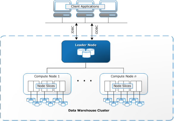
Under the hood, AWS Redshift is based on PostgreSQL 8.0.2. The architecture consist of 1 leader node – a node which is responsible for managing the communications with the clients, developing the execution plan and then distributing the compiled code to the compute nodes-, and 1 or more compute nodes that are exetung the code and then sending back the result to the leader node for aggregation. The compute nodes can have either 2-cores, 15GB RAM and 2 TB storage node (dubbed as XL node) or a 16-cores, 120 GB RAM and 16 TB storage node (dubbed as 8XL node). More details about the Redshift archtecture can be found at http://docs.aws.amazon.com/redshift/latest/dg/c_internal_arch_system_operation.html

AWS-Redshift-Arch

Launching a cluster

The easiest way to launch a cluster is via AWS console.

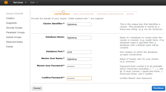
We need to define the basic attributes like cluster identifier, database name, database port, master username and password:

AWS-RedShift1

Then we need to select the node type (XL or 8XL) and the number of compute nodes. A cluster can be single or multi-node, the minimum config is a one XL node cluster, while the maximum config is sixteen 8XL nodes – you can do the math in terms of cores, memory and storage.

AWS-Redshift2

Then we can configure additional parameters (like database encyption or security groups)

AWS-Redshift4

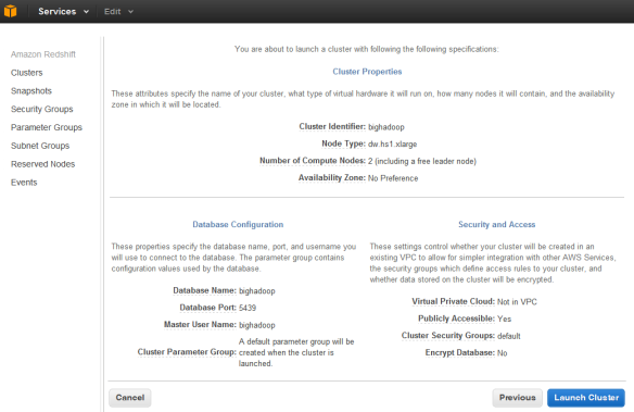
We can then review the configuration and are ready to launch the service:

AWS-RedShift5

The status will be first “creating” for a while then it will become “available”. This is when the JDBC url will become known and can be used for configuring the clients.

AWS-RedShift8

In order to make the service accessible, we need to configure the security options (either a security group – if Redshift is going to be accessed from EC2 – or a CIDR/IP (Classless- Inter-Domain Routing IP range)  – if Redshift is to be accessed from public Internet.  The system will automatically recognise the IP address of the client connected to AWS console.

AWS-RedShift6

And that is it! From then on the client can be connected to the Redshift cluster.

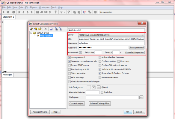
We used SQLWorkbench to test the service, the same way as suggested by AWS Redshift documentation. It is a Java based open source SQL tool. The connection parameters are the standard JDBC attributes:

AWS-Redshift9

The PostgreSQL version can be checked using

select version();

version
PostgreSQL 8.0.2 on i686-pc-linux-gnu, compiled by GCC gcc (GCC) 3.4.2 20041017 (Red Hat 3.4.2-6.fc3), Redshift 1.0.546

We tested the service with Amazon stock prices downloaded from Yahoo Finance.

The content has been uploaded to a S3 bucket called stockprice (S3://stockprice/amzn.csv). We had to make it accessible for everyone to read. (open/download).

Then we could create the appropriate table using standard SQL command:

CREATE TABLE stockprice (
     stockdate date not null,
     stockopen decimal(6,2),
     stockhigh decimal(6,2),
     stocklow decimal(6,2),
     stockclose decimal(6,2),
     stockvolume integer,
     stockadjclose decimal(6,2)
     );

Table 'stockprice' created

Execution time: 0.15s

desc stockprice
COLUMN_NAME	DATA_TYPE	PK	NULLABLE	DEFAULT	AUTOINCREMENT	REMARKS	POSITION
stockdate	date	NO	YES		NO		1
stockopen	numeric(6,2)	NO	YES		NO		2
stockhigh	numeric(6,2)	NO	YES		NO		3
stocklow	numeric(6,2)	NO	YES		NO		4
stockclose	numeric(6,2)	NO	YES		NO		5
stockvolume	integer	NO	YES		NO		6
stockadjclose	numeric(6,2)	NO	YES		NO		7

To load the data into stockprice table, we had to use copy command with the S3 source file (it could also be an Amazon DynamoDB source).

copy stockprice from 's3://stockprices/amzn.csv' CREDENTIALS 'aws_access_key_id=XXXXXXX;aws_secret_access_key=XXXXXXX' delimiter ',';

If there is any error during the load operation, it can be verified by running a select statement on the stl_load_errors table. (e.g. incorrect data format).

And then we can run our SQL statements to analyse the data.

select * from stockprice order by stockadjclose desc limit 100;

stockdate	stockopen	stockhigh	stocklow	stockclose	stockvolume	stockadjclose
2013-01-25	275.00	284.72	274.40	283.99	4968100	283.99
2013-01-28	283.78	284.48	274.40	276.04	4321400	276.04
2013-03-05	274.00	276.68	269.99	275.59	3686200	275.59
2013-03-13	275.24	276.50	272.64	275.10	1884200	275.10
2013-03-08	275.00	275.44	271.50	274.19	1879800	274.19
2013-03-12	271.00	277.40	270.36	274.13	3246200	274.13
2013-03-07	274.10	274.80	271.85	273.88	1939000	273.88
2013-03-06	275.76	276.49	271.83	273.79	2050700	273.79
2013-01-24	269.37	276.65	269.37	273.46	3417000	273.46
2013-03-04	265.36	273.30	264.14	273.11	3453000	273.11
2013-01-30	283.00	284.20	267.11	272.76	13075400	272.76
2013-01-14	268.00	274.26	267.54	272.73	4275000	272.73
2013-01-18	270.83	274.50	269.60	272.12	2942000	272.12
2013-01-15	270.68	272.73	269.30	271.90	2326900	271.90
2013-03-11	273.43	273.99	270.40	271.24	1904900	271.24

AWS console supports various management functions of the cluster, we can reboot the cluster, we can modify parameters, we can resize it by defining different node type (XL->8XL) or decreasing/increasing the number of nodes. We can also delete the cluster via AWS console.
AWS-Redshift11

Conclusion

Amazon Web Services Redshift is another big step to make cloud services available for enterprise computing. It offers a data warehouse capability with minimal effort to start up and scale as operations demand. It is a great complement to other database services such as DynamoDB for NoSQL requirements and RDS for relational database services.

R and Hadoop Data Analysis – RHadoop


Introduction

R is a programming language and a software suite used for data analysis, statistical computing and data visualization. It is highly extensible and has object oriented features and strong graphical capabilities. At its heart R is an interpreted language and comes with a command line interpreter – available for Linux, Windows and Mac machines – but there are IDEs as well to support development like RStudio or JGR.

R and Hadoop can complement each other very well, they are a natural match in big data analytics and visualization. One of the most well-known R packages to support Hadoop functionalities is RHadoop that was developed by RevolutionAnalytics.

Installing RHadoop

RHadoop is a collection of three R packages: rmr, rhdfs and rhbase. rmr package provides Hadoop MapReduce functionality in R, rhdfs provides HDFS file management in R and rhbase provides HBase database management from within R.

To install these R packages, first we need to install R base package. On Ubuntu 12.04 LTS we can do it running:

$ sudo apt-get install r-base

Then we need to install RHadoop packages with their dependencies.  rmr requires RCpp, RJSONIO, digest, functional, stringr and plyr, while rhdfs requires rJava.

As part of the installation, we need to reconfigure Java for rJava package and we also need to set HADOOP_CMD variable for rhdfs package. The installation requires the corresponding tar.gz archives to be downloaded and then we can run R CMD INSTALL command with sudo privileges.

sudo R CMD INSTALL Rcpp Rcpp_0.10.2.tar.gz
sudo R CMD INSTALL RJSONIO RJSONIO_1.0-1.tar.gz
sudo R CMD INSTALL digest digest_0.6.2.tar.gz
sudo R CMD INSTALL functional functional_0.1.tar.gz
sudo R CMD INSTALL stringr stringr_0.6.2.tar.g
sudo R CMD INSTALL plyr plyr_1.8.tar.gz
sudo R CMD INSTALL rmr rmr2_2.0.2.tar.gz

sudo JAVA_HOME=/home/istvan/jdk1.6.0_38/jre R CMD javareconf
sudo R CMD INSTALL rJava rJava_0.9-3.tar.gz 
sudo HADOOP_CMD=/home/istvan/hadoop/bin/hadoop R CMD INSTALL rhdfs rhdfs_1.0.5.tar.gz 
sudo R CMD INSTALL rhdfs rhdfs_1.0.5.tar.gz

Getting started with RHadoop

In principle, RHadoop MapReduce is a similar operation to R lapply function that applies a function over a list or vector.

Without mapreduce function we could write a simple R code to double all the numbers from 1 to 100:

> ints = 1:100
> doubleInts = sapply(ints, function(x) 2*x)
> head(doubleInts)
[1]  2  4  6  8 10 12

With RHadoop rmr package we could use mapreduce function to implement the same calculations – see doubleInts.R script:

Sys.setenv(HADOOP_HOME="/home/istvan/hadoop")
Sys.setenv(HADOOP_CMD="/home/istvan/hadoop/bin/hadoop")

library(rmr2)
library(rhdfs)

ints = to.dfs(1:100)
calc = mapreduce(input = ints,
                   map = function(k, v) cbind(v, 2*v))

from.dfs(calc)

$val
         v    
  [1,]   1   2
  [2,]   2   4
  [3,]   3   6
  [4,]   4   8
  [5,]   5  10
.....

If we want to run HDFS filesystem commands from R, we first need to initialize rhdfs using hdfs.init() function, then we can run the well-known ls, rm, mkdir, stat, etc commands:

> hdfs.init()
> hdfs.ls("/tmp")
  permission  owner      group size          modtime               file
1 drwxr-xr-x istvan supergroup    0 2013-02-25 21:59    /tmp/RtmpC94L4R
2 drwxr-xr-x istvan supergroup    0 2013-02-25 21:49 /tmp/hadoop-istvan
> hdfs.stat("/tmp")
      perms isDir block replication  owner      group size              modtime path
1 rwxr-xr-x  TRUE     0           0 istvan supergroup    0 45124-08-29 23:58:48 /tmp

Data analysis with RHadoop

The following example demonstrates how to use RHadoop for data analysis. Let us assume that we need to determine how many countries have greater GDP than Apple Inc.’s revenue in 2012. (It was 156,508 millions USD, see more details  http://www.google.com/finance?q=NASDAQ%3AAAPL&fstype=ii&ei=5eErUcCpB8KOwAOkQQ)

GDP data can be downloaded from Worldbank data catalog site. The data needs to be adjusted to be suitable for MapReduce algorithm. The final format that we used for data analysis is as follows (where the last column is the GDP of the given country in millions USD):

Country Code,Number,Country Name,GDP,
USA,1,United States,14991300
CHN,2,China,7318499
JPN,3,Japan,5867154
DEU,4,Germany,3600833
FRA,5,France,2773032
....

The gdp.R script looks like this:

Sys.setenv(HADOOP_HOME="/home/istvan/hadoop")
Sys.setenv(HADOOP_CMD="/home/istvan/hadoop/bin/hadoop")

library(rmr2)
library(rhdfs)

setwd("/home/istvan/rhadoop/blogs/")
gdp <- read.csv("GDP_converted.csv")
head(gdp)

hdfs.init()
gdp.values <- to.dfs(gdp)

# AAPL revenue in 2012 in millions USD
aaplRevenue = 156508

gdp.map.fn <- function(k,v) {
key <- ifelse(v[4] < aaplRevenue, "less", "greater")
keyval(key, 1)
}

count.reduce.fn <- function(k,v) {
keyval(k, length(v))
}

count <- mapreduce(input=gdp.values,
                   map = gdp.map.fn,
                   reduce = count.reduce.fn)

from.dfs(count)

R will initiate a Hadoop streaming job to process the data using mapreduce algorithm.

packageJobJar: [/tmp/Rtmp4llUjl/rmr-local-env1e025ac0444f, /tmp/Rtmp4llUjl/rmr-global-env1e027a86f559, /tmp/Rtmp4llUjl/rmr-streaming-map1e0214a61fa5, /tmp/Rtmp4llUjl/rmr-streaming-reduce1e026da4f6c9, /tmp/hadoop-istvan/hadoop-unjar1158187086349476064/] [] /tmp/streamjob430878637581358129.jar tmpDir=null
13/02/25 22:28:12 INFO mapred.FileInputFormat: Total input paths to process : 1
13/02/25 22:28:12 INFO streaming.StreamJob: getLocalDirs(): [/tmp/hadoop-istvan/mapred/local]
13/02/25 22:28:12 INFO streaming.StreamJob: Running job: job_201302252148_0006
13/02/25 22:28:12 INFO streaming.StreamJob: To kill this job, run:
13/02/25 22:28:12 INFO streaming.StreamJob: /home/istvan/hadoop-1.0.4/libexec/../bin/hadoop job  -Dmapred.job.tracker=localhost:9001 -kill job_201302252148_0006
13/02/25 22:28:12 INFO streaming.StreamJob: Tracking URL: http://localhost:50030/jobdetails.jsp?jobid=job_201302252148_0006
13/02/25 22:28:13 INFO streaming.StreamJob:  map 0%  reduce 0%
13/02/25 22:28:25 INFO streaming.StreamJob:  map 100%  reduce 0%
13/02/25 22:28:37 INFO streaming.StreamJob:  map 100%  reduce 100%
13/02/25 22:28:43 INFO streaming.StreamJob: Job complete: job_201302252148_0006
13/02/25 22:28:43 INFO streaming.StreamJob: Output: /tmp/Rtmp4llUjl/file1e025f146f8f

Then we will get the data saying how many countries have greater and how many contries have less GDP than Apple Inc.’s revenue in year 2012. The result is that 55 countries had greater GDP than Apple and 138 countries had less.

$key
   GDP      
1  "greater"
56 "less"   

$val
[1]  55 138

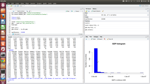
The following screenshot from RStudio shows the histogram of GDPs – there are 15 countries having more than 1,000 millions USD GDP; 1 country is in the range of 14,000 – 15,000 millions USD, 1 country is in the range of 7,000 – 8,000 millions USD and 1 country is in the range of 5,000 – 6,000 USD.

GDP-histogram

Conclusion

If someone needs to combine strong data analytics and visualization features  with big data capabilities supported by Hadoop, it is certainly worth to have a closer look at RHadoop features. It has packages to integrate R with MapReduce, HDFS and HBase, the key components of the Hadoop ecosystem. For more details, please read the R and Hadoop Big Data Analytics whitepaper.

Prediction API – Machine Learning from Google


Introduction

One of the exciting APIs among the 50+ APIs offered by Google is the Prediction API. It provides pattern matching and machine learning capabilities like recommendations or categorization. The notion is similar to the machine learning capabilities that we can see in other solutions (e.g. in Apache Mahout): we can train the system with a set of training data and then the applications based on Prediction API can recommend (“predict”) what products the user might like or  they can categories spams, etc.

In this post we go through an example how to categorize SMS messages – whether they are spams or valuable texts (“hams”).

Using Prediction API

In order to be able to use Prediction API, the service needs to be enabled via Google API console. To upload training data, Prediction API also requires Google Cloud Storage.

The dataset  used in this post is from UCI Machine Learning Repository.  UCI Machine Learning repository has 235 datasets publicly available, this post is based on SMS Spam Collections dataset.

To upload the training data first we need to create a bucket in Google Cloud Storage. From Google API console we need to click on Google Cloud Storage and then on Google Cloud Storage Manager: This will open a webpage whe we can create new buckets and upload or delete files.

GoogleStorage2

The UCI SMS Spam Collection file is not suitable as is for Prediction API, it needs to be converted into the following format (the categories – ham/spam – need to be quoted as well as the SMS text):

“ham” “Go until jurong point, crazy.. Available only in bugis n great world la e buffet… Cine there got amore wat…”

GoogleStorage4

Google Prediction API offers a handful of commands that can be invoked via REST interface. The simplest way of testing Prediction API is to use Prediction API explorer.

GooglePrediction1

Once the training data is available on Google Cloud Storage, we can start training the machine learning system behind Prediction API. To begin training our model, we need to run prediction.trainedmodels.insert. All commands require authentication, it is based on OAuth 2.0 standard.

GooglePrediction2

In the insert menu we need to specify the fields that we want to be included in the response.  In the request body we need to define an id (this will be used as a reference to the model in the commands used later on), a storageDataLocation where we have the training data uploaded (the Google Cloud Storage path) and the modelType (could be regression or classification, for spam filtering it is classification):

GooglePrediction-SpamInsert1

The training runs for a while, we can check the status using prediction.trainedmodels.get command. The status field is going to be RUNNING and then will be changed to DONE, once the training is finished.

GooglePrediction-SpamGet1

GooglePrediction-SpamGet2

Now we are ready to run our test against the machine learning system and it is going to classify whether the given text is spam or ham. The Prediction API command for this action is prediction.trainedmodels.predict. In the id field we have to refer to the id that we defined for the  prediction.trainedmodels.insert command (bighadoop-00001) and we also need to specify the request body – input will be csvInstance and then we enter the text that we want to get categorized (e.g. “Free entry”)

GooglePrediction-SpamPredict1

The system then returns with the category (spam) and the score (0.822158 for spam, 0.177842 for ham):

GooglePrediction-SpamPredict2

Google Prediction API libraries

Google also offers a featured sample application that includes all the code required to run it on Google App Engine. It is called Try-Prediction and the code is written in Python and also in Java. The application can be tested at http://try-prediction.appspot.com.

For instance, if we enter a quote for the Language Detection model from Niels Bohr: “Prediction is very difficult, especially if it’s about the future.”, it will return that it is likely to be an English text (54,4%).

TryPrediction

The key part of the Python code is in predict.py:

class PredictAPI(webapp.RequestHandler):
  '''This class handles Ajax prediction requests, i.e. not user initiated
     web sessions but remote procedure calls initiated from the Javascript
     client code running the browser.
  '''

  def get(self):
    try:
      # Read server-side OAuth 2.0 credentials from datastore and
      # raise an exception if credentials not found.
      credentials = StorageByKeyName(CredentialsModel, USER_AGENT, 
                                    'credentials').locked_get()
      if not credentials or credentials.invalid:
        raise Exception('missing OAuth 2.0 credentials')

      # Authorize HTTP session with server credentials and obtain  
      # access to prediction API client library.
      http = credentials.authorize(httplib2.Http())
      service = build('prediction', 'v1.4', http=http)
      papi = service.trainedmodels()

      # Read and parse JSON model description data.
      models = parse_json_file(MODELS_FILE)

      # Get reference to user's selected model.
      model_name = self.request.get('model')
      model = models[model_name]

      # Build prediction data (csvInstance) dynamically based on form input.
      vals = []
      for field in model['fields']:
        label = field['label']
        val = str(self.request.get(label))
        vals.append(val)
      body = {'input' : {'csvInstance' : vals }}
      logging.info('model:' + model_name + ' body:' + str(body))

      # Make a prediction and return JSON results to Javascript client.
      ret = papi.predict(id=model['model_id'], body=body).execute()
      self.response.out.write(json.dumps(ret))

    except Exception, err:
      # Capture any API errors here and pass response from API back to
      # Javascript client embedded in a special error indication tag.
      err_str = str(err)
      if err_str[0:len(ERR_TAG)] != ERR_TAG:
        err_str = ERR_TAG + err_str + ERR_END
      self.response.out.write(err_str)

The Java version of Prediction web application is as follows:

public class PredictServlet extends HttpServlet {

  @Override
  protected void doGet(HttpServletRequest request,
                       HttpServletResponse response) throws ServletException, 
                                                            IOException {
    Entity credentials = null;
    try {
      // Retrieve server credentials from app engine datastore.
      DatastoreService datastore = 
        DatastoreServiceFactory.getDatastoreService();
      Key credsKey = KeyFactory.createKey("Credentials", "Credentials");
      credentials = datastore.get(credsKey);
    } catch (EntityNotFoundException ex) {
      // If can't obtain credentials, send exception back to Javascript client.
      response.setContentType("text/html");
      response.getWriter().println("exception: " + ex.getMessage());
    }

    // Extract tokens from retrieved credentials.
    AccessTokenResponse tokens = new AccessTokenResponse();
    tokens.accessToken = (String) credentials.getProperty("accessToken");
    tokens.expiresIn = (Long) credentials.getProperty("expiresIn");
    tokens.refreshToken = (String) credentials.getProperty("refreshToken");
    String clientId = (String) credentials.getProperty("clientId");
    String clientSecret = (String) credentials.getProperty("clientSecret");
    tokens.scope = IndexServlet.scope;

    // Set up the HTTP transport and JSON factory
    HttpTransport httpTransport = new NetHttpTransport();
    JsonFactory jsonFactory = new JacksonFactory();

    // Get user requested model, if specified.
    String model_name = request.getParameter("model");

    // Parse model descriptions from models.json file.
    Map models = 
      IndexServlet.parseJsonFile(IndexServlet.modelsFile);

    // Setup reference to user specified model description.
    Map selectedModel = 
      (Map) models.get(model_name);
    
    // Obtain model id (the name under which model was trained), 
    // and iterate over the model fields, building a list of Strings
    // to pass into the prediction request.
    String modelId = (String) selectedModel.get("model_id");
    List params = new ArrayList();
    List<Map > fields = 
      (List<Map >) selectedModel.get("fields");
    for (Map field : fields) {
      // This loop is populating the input csv values for the prediction call.
      String label = field.get("label");
      String value = request.getParameter(label);
      params.add(value);
    }

    // Set up OAuth 2.0 access of protected resources using the retrieved
    // refresh and access tokens, automatically refreshing the access token 
    // whenever it expires.
    GoogleAccessProtectedResource requestInitializer = 
      new GoogleAccessProtectedResource(tokens.accessToken, httpTransport, 
                                        jsonFactory, clientId, clientSecret, 
                                        tokens.refreshToken);

    // Now populate the prediction data, issue the API call and return the
    // JSON results to the Javascript AJAX client.
    Prediction prediction = new Prediction(httpTransport, requestInitializer, 
                                           jsonFactory);
    Input input = new Input();
    InputInput inputInput = new InputInput();
    inputInput.setCsvInstance(params);
    input.setInput(inputInput);
    Output output = 
      prediction.trainedmodels().predict(modelId, input).execute();
    response.getWriter().println(output.toPrettyString());
  }
}

Besides Python and Java support, Google also offers .NET, Objective-C, Ruby, Go, JavaScript, PHP, etc. libraries for Prediction API.

Mahout on Windows Azure – Machine Learning Using Microsoft HDInsight


Introduction

Our last post was about Microsoft and Hortonworks joint effort to deliver Hadoop on Microsoft Windows Azure dubbed HDInsight. One of the key Microsoft HDInsight components is Mahout, a scalable machine learning library that provides a number of algorithms relying on the Hadoop platform. Machine learning supports a wide range of use cases from email spam filtering to fraud detection to recommending books or movies, similar to Amazon.com features.These algorithms can be divided into three main categories: recommenders/collaborative filtering, categorization and clustering. More details about these algorithms can be read on Apache Mahout wiki.

Recommendation engine on Azure

A standard recommender example in machine learning is a movie recommender. Surprisingly enough this example is not among the provided HDInsight examples so we need to implement it on our own using mahout-0.5 components.

The movie recommender is an item based recommendation algorithm: the key concept is that having a large dataset of users, movies and values indicating how much a user liked that particular movie, the algorithm will recommend movies to the users. A commonly used dataset for movie recommendation is from GroupLens.

The downloadable file that is part of the 100K dataset (u.data) is not suitable for Mahout as is because its format is like:

user item value timestamp
196 242 3 881250949
186 302 3 891717742
22 377 1 878887116
....

Mahout requires the data to be in the following format: userid,itemid,value
so the content has to be converted to

196,242,3
186,302,3
22,377,1
....

There is no web based console to execute Mahout on Azure, we need to go to Remote Desktop to download the RDP configuration and then login to Azure headnode via RDP. Then we have to run Hadoop command line to get a prompt.

c:>c:\apps\dist\hadoop-1.1.0-SNAPSHOT\bin\hadoop jar c:\apps\dist\mahout-0.5\mahout-examples-0.5-job.jar org.apache.mahout.driver.MahoutDriver recommenditembased --input recommend.csv --output recommendout --tempDir recommendtmp --usersFile user-ids.txt --similarityClassname SIMILARITY_EUCLIDEAN_DISTANCE --numRecommendations 5

The standard mahout.cmd seems to have a few bugs, if we run mahout.cmd then it will throw an error complaining about java usage. I had to modify the file to remove setting HADOOP_CLASSPATH envrionment variable, see the changes in bold-italic:

@rem run it
if not [%MAHOUT_LOCAL%] == [] (
    echo "MAHOUT_LOCAL is set, running locally"
    %JAVA% %JAVA_HEAP_MAX% %MAHOUT_OPTS% -classpath %MAHOUT_CLASSPATH% %CLASS% %*
) else (
    if [%MAHOUT_JOB%] == [] (
        echo "ERROR: Could not find mahout-examples-*.job in %MAHOUT_HOME% or %MAHOUT_HOME%\examples\target"
        goto :eof
    ) else (
@rem  set HADOOP_CLASSPATH=%MAHOUT_CLASSPATH%
        if /I [%1] == [hadoop] (
            echo Running: %HADOOP_HOME%\bin\%*
            call %HADOOP_HOME%\bin\%*
        ) else (
            echo Running: %HADOOP_HOME%\bin\hadoop jar %MAHOUT_JOB% %CLASS% %*
            call %HADOOP_HOME%\bin\hadoop jar %MAHOUT_JOB% %CLASS% %*
        )
    )
)

After this change we can run mahout as expected:

c:\apps\dist\mahout-0.5\bin>mahout.cmd recommenditembased --input recommend.csv --output recommendout --tempDir recommendtmp --usersFile user-ids.txt --similarityClassname SIMILARITY_EUCLIDEAN_DISTANCE --numRecommendations 5

Input argument defines the path to the input directory, output argument determines the path to output directory.

The numRecommendations means the number of recommendations per user.

The usersFile defines the users to recommend for (in our case it contained 3 users only, 112, 286, 310:

c:>hadoop fs -cat user-ids.txt
112
286
301

The similarityClass is the name of the distributed similarity class and it can be SIMILARITY_EUCLIDEAN_DISTANCE,  SIMILARITY_LOGLIKELIHOOD, SIMILARITY_PEARSON_CORRELATION, etc. This class determine the algorithm to calculate similarities between the items.

The execution of MapReduce tasks can be monitored via Hadoop MapReduce admin console:

mahout-recommender-console

mahout-recommender-console1

Once the job is finished, we need to use hadoop filesystem commands to display the output file produced by the RecommenderJob:

c:\apps\dist\hadoop-1.1.0-SNAPSHOT>hadoop fs -ls .
Found 5 items
drwxr-xr-x   - istvan supergroup          0 2012-12-21 11:00 /user/istvan/.Trash

-rw-r--r--   3 istvan supergroup    1079173 2012-12-23 22:40 /user/istvan/recomm
end.csv
drwxr-xr-x   - istvan supergroup          0 2012-12-24 12:24 /user/istvan/recomm
endout
drwxr-xr-x   - istvan supergroup          0 2012-12-24 12:22 /user/istvan/recomm
endtmp
-rw-r--r--   3 istvan supergroup         15 2012-12-23 22:40 /user/istvan/user-i
ds.txt

c:\apps\dist\hadoop-1.1.0-SNAPSHOT>hadoop fs -ls recommendout
Found 3 items
-rw-r--r--   3 istvan supergroup          0 2012-12-24 12:24 /user/istvan/recomm
endout/_SUCCESS
drwxr-xr-x   - istvan supergroup          0 2012-12-24 12:23 /user/istvan/recomm
endout/_logs
-rw-r--r--   3 istvan supergroup        153 2012-12-24 12:24 /user/istvan/recomm
endout/part-r-00000

c:\apps\dist\hadoop-1.1.0-SNAPSHOT>hadoop fs -cat recommendout/part-r*
112     [1228:5.0,1473:5.0,1612:5.0,1624:5.0,1602:5.0]
286     [1620:5.0,1617:5.0,1615:5.0,1612:5.0,1611:5.0]
301     [1620:5.0,1607:5.0,1534:5.0,1514:5.0,1503:5.0]

Thus the RecommenderJob recommends item 1228, 1473, 1612, 1624 and 1602 to user 112; item 1620, 1617, 1615, 1612 and 1611 for user 286 and 1620, 1607, 1534, 1514 and 1503 for user 301, respectively.

For those inclined to theory and scientific papers, I suggest to read the paper from Sarwar, Karypis, Konstand and Riedl that provides the background of the item based recommendation algorithms.

Mahout examples on Azure

Hadoop on Azure comes with two predefined examples: one for classification, one for clustering. They require command line to be executed – a smilar way as described above for the item based recommendation engine.

mahout

The classification demo is based on naive Bayes classifier- first you need to train your classifier with a set of known data and then you can run the algorithm on the actual data set. This concept is called supervised learning.

To run the classification example we need to download the 20news-bydate.tar.gz file from http://people.csail.mit.edu/jrennie/20Newsgroups/20news-bydate.tar.gz and unzip it under mahout-0.5/examples/bin/work directory. The data set has two subsets, one for training the classifier and the other one to run the test. Then we can run the command:

c:\apps\dist\mahout-0.5\examples\bin> build-20news-bayes.cmd

This will kick off the Hadoop MapReduce job and after a while it will spit out the confusion matrix based on Bayes algorithm. The confusion matrix will tell us what categories were correctly identified by the classifier and what were incorrect.

For instance, it has a category called rec.motorcycles (column a), and the classifier correctly identified 381 items out of 398 belonging to this cathegory, while it defined 9 items incorrectly as belonging to rec.autos (column f), 2 items incorrectly as belonging to sci.electronics (column n), etc.

WORK_PATH=c:\apps\dist\mahout-0.5\examples\bin\work\20news-bydate\
Running: c:\apps\dist\hadoop-1.1.0-SNAPSHOT\bin\hadoop jar c:\apps\dist\mahout-0
.5\bin\..\\mahout-examples-0.5-job.jar org.apache.mahout.driver.MahoutDriver tes
tclassifier   -m examples/bin/work/20news-bydate/bayes-model   -d examples/bin/w
ork/20news-bydate/bayes-test-input   -type bayes   -ng 1   -source hdfs   -metho
d "mapreduce"

12/12/24 17:55:58 INFO mapred.JobClient:     Map output records=7532
12/12/24 17:55:59 INFO bayes.BayesClassifierDriver: ============================
===========================
Confusion Matrix
-------------------------------------------------------
a       b       c       d       e       f       g       h       i       j
k       l       m       n       o       p       q       r       s       t
u       <--Classified as
381     0       0       0       0       9       1       0       0       0
1       0       0       2       0       1       0       0       3       0
0        |  398         a     = rec.motorcycles
1       284     0       0       0       0       1       0       6       3
11      0       66      3       0       1       6       0       4       9
0        |  395         b     = comp.windows.x
2       0       339     2       0       3       5       1       0       0
0       0       1       1       12      1       7       0       2       0
0        |  376         c     = talk.politics.mideast
4       0       1       327     0       2       2       0       0       2
1       1       0       5       1       4       12      0       2       0
0        |  364         d     = talk.politics.guns
7       0       4       32      27      7       7       2       0       12
0       0       6       0       100     9       7       31      0       0
0        |  251         e     = talk.religion.misc
10      0       0       0       0       359     2       2       0       1
3       0       1       6       0       1       0       0       11      0
0        |  396         f     = rec.autos
0       0       0       0       0       1       383     9       1       0
0       0       0       0       0       0       0       0       3       0
0        |  397         g     = rec.sport.baseball
1       0       0       0       0       0       9       382     0       0
0       0       1       1       1       0       2       0       2       0
0        |  399         h     = rec.sport.hockey
2       0       0       0       0       4       3       0       330     4
4       0       5       12      0       0       2       0       12      7
0        |  385         i     = comp.sys.mac.hardware
0       3       0       0       0       0       1       0       0       368
0       0       10      4       1       3       2       0       2       0
0        |  394         j     = sci.space
0       0       0       0       0       3       1       0       27      2
291     0       11      25      0       0       1       0       13      18
0        |  392         k     = comp.sys.ibm.pc.hardware
8       0       1       109     0       6       11      4       1       18
0       98      1       3       11      10      27      1       1       0
0        |  310         l     = talk.politics.misc
0       11      0       0       0       3       6       0       10      6
11      0       299     13      0       2       13      0       7       8
0        |  389         m     = comp.graphics
6       0       1       0       0       4       2       0       5       2
12      0       8       321     0       4       14      0       8       6
0        |  393         n     = sci.electronics
2       0       0       0       0       0       4       1       0       3
1       0       3       1       372     6       0       2       1       2
0        |  398         o     = soc.religion.christian
4       0       0       1       0       2       3       3       0       4
2       0       7       12      6       342     1       0       9       0
0        |  396         p     = sci.med
0       1       0       1       0       1       4       0       3       0
1       0       8       4       0       2       369     0       1       1
0        |  396         q     = sci.crypt
10      0       4       10      1       5       6       2       2       6
2       0       2       1       86      15      14      152     0       1
0        |  319         r     = alt.atheism
4       0       0       0       0       9       1       1       8       1
12      0       3       6       0       2       0       0       341     2
0        |  390         s     = misc.forsale
8       5       0       0       0       1       6       0       8       5
50      0       40      2       1       0       9       0       3       256
0        |  394         t     = comp.os.ms-windows.misc
0       0       0       0       0       0       0       0       0       0
0       0       0       0       0       0       0       0       0       0
0        |  0           u     = unknown
Default Category: unknown: 20

12/12/24 17:55:59 INFO driver.MahoutDriver: Program took 129826 ms

c:\apps\dist\mahout-0.5\examples\bin

Again for those interested in theory and scientific papers, I suggest to read the following webpage.

Microsoft and Hadoop – Windows Azure HDInsight


Introduction

Traditionally Microsoft Windows used to be a sort of stepchild in Hadoop world – the ‘hadoop’ command to manage actions from command line and the startup/shutdown scripts were written in Linux/*nix in mind assuming bash. Thus if you wanted to run Hadoop on Windows, you had to install cygwin. Also Apache Hadoop document states the following (quotes from Hadoop R1.1.0 documentation):
“•GNU/Linux is supported as a development and production platform. Hadoop has been demonstrated on GNU/Linux clusters with 2000 nodes
•Win32 is supported as a development platform. Distributed operation has not been well tested on Win32, so it is not supported as a production platform.”

Microsoft and Hortonworks joined their forces to make Hadoop available on Windows Server for on-premise deployments as well as on Windows Azure to support big data in the cloud, too.

This post covers Windows Azure HDInsight (Hadoop on Azure, see https://www.hadooponazure.com) . As of writing, the service requires an invitation to participate in the CTP (Community Technology Preview) but the invitation process is very efficiently managed – after filling in the survey, I received the service access code within a couple of days.

New Cluster Request

The first step is to request a new cluster, you need to define the cluster name and the credentials to be able to login to the headnode. By default the cluster consists of 3 nodes.

After a few minutes, you will have a running cluster,  then click on the “Go to Cluster” link to navigate to the main page.

WordCount with HDInsight on  Azure

No Hadoop test is complete without the standard WordCount application – Microsoft Azure HDInsight provides an example file (davinci.txt) and the Java jar file to run wordcount  – the Hello World of Hadoop.

First you need to go to the JavaScript console to upload the text file using fs.put():

js> fs.put()

Choose File ->  Browse
Destination: /user/istvan/example/data/davinci

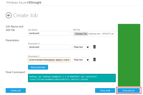
Create a Job:

CreateJob

The actual command that Microsoft Azure HDInsight executes is as follows:

c:\apps\dist\hadoop-1.1.0-SNAPSHOT\bin\hadoop.cmd jar c:\apps\Jobs\templates\634898986181212311.hadoop-examples-1.1.0-SNAPSHOT.jar wordcount /user/istvan/example/data/davinci davinci-output

You can validate the output from JavaScript console:

js> result = fs.read("davinci-output")
"(Lo)cra"	1
"1490	1
"1498,"	1
"35"	1
"40,"	1
"AS-IS".	1
"A_	1
"Absoluti	1
"Alack!	1

Microsoft HDInsight Streaming – Hadoop job in C#

Hadoop Streaming is a utility to support running external map and reduce jobs. These external jobs can be written in various programming languages such as Python or Ruby – should we talk about Microsoft HDInsight, the example better be based on .NET C#…

The demo application for C# streaming is again a wordcount example using the imitation of Unix cat and wc commands. You could run the demo from the “Samples” tile but I prefer to demonstrate Hadoop Streaming from the command line to have a closer look at what is going on under the hood.

In order to run Hadoop command line from Windows cmd prompt, you need to login to the HDInsight headnode using Remote Desktop. First you need to click on “Remote Desktop” tile, then login the remote node using the credentials you defined at cluster creation time. Once you logged in, click on Hadoop Coomand Line shortcut.

In Hadoop Command Line, go to the Hadoop distribution directory (As of writing this post, Microsoft Azure HDInsight is based on Hadoop 1.1.0):

c:> cd \apps\dist
c:> hadoop fs -get /example/apps/wc.exe .
c:> hadoop fs -get /example/apps/cat.exe .
c:> cd \apps\dist\hadoop-1.1.0-SNAPSHOT
c:\apps\dist\hadoop-1.1.0-SNAPSHOT> hadoop jar lib\hadoop-streaming.jar -input "/user/istvan/example/data/davinci" -output "/user/istvan/example/dataoutput" -mapper "..\..\jars\cat.exe" -reducer "..\..\jars\wc.exe" -file "c:\Apps\dist\wc.exe" -file "c:\Apps\dist\cat.exe"

The C# code for wc.exe is as follows:

using System;
using System.IO;
using System.Linq;

namespace wc
{
    class wc
    {
        static void Main(string[] args)
        {
            string line;
            var count = 0;

            if (args.Length > 0){
                Console.SetIn(new StreamReader(args[0]));
            }

            while ((line = Console.ReadLine()) != null) {
                count += line.Count(cr => (cr == ' ' || cr == '\n'));
            }
            Console.WriteLine(count);
        }
    }
}

And the code for cat.exe is:

using System;
using System.IO;

namespace cat
{
    class cat
    {
        static void Main(string[] args)
        {
            if (args.Length > 0)
            {
                Console.SetIn(new StreamReader(args[0])); 
            }

            string line;
            while ((line = Console.ReadLine()) != null) 
            {
                Console.WriteLine(line);
            }

        }

    }
}

Interactive console

Microsoft Azure HDInsight comes with two types of interactive console: one is the standard Hadoop Hive console, the other one is unique in Hadoop world, it is based on JavaScript.

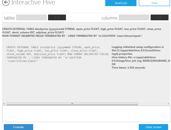
Let us start with Hive. You need to upload your data using the javascript fs.put() method as described above. Then you can create your Hive table and run a select query as follows :

CREATE TABLE stockprice (yyyymmdd STRING, open_price FLOAT, high_price FLOAT, low_price FLOAT, close_price FLOAT, stock_volume INT, adjclose_price FLOAT)
row format delimited fields terminated by ',' lines terminated by '\n' location '/user/istvan/input/';

select yyyymmdd, high_price, stock_volume from stockprice order by high_price desc;

InteractiveHive

InteractiveHive-Select

The other flavor of HDInsight interactive console is based on JavaScript – as said before, this is a unique offering from Microsoft – in fact, the JavaScript commands are converted to Pig statements.

JavascriptConsole

The syntax resembles a kind of LINQ style query, though not the same:

js> pig.from("/user/istvan/input/goog_stock.csv", "date,open,high,low,close,volume,adjclose", ",").select("date, high, volume").orderBy("high DESC").to("result")

js> result = fs.read("result")
05/10/2012	774.38	2735900
04/10/2012	769.89	2454200
02/10/2012	765.99	2790200
01/10/2012	765	3168000
25/09/2012	764.89	6058500

Under the hood

Microsoft and Hortonworks have re-implemented the key binaries (namenode, jobtracker, secondarynamenode, datanode, tasktracker) as executables (exe files) and they are running as services in the background. The key ‘hadoop’ command – which is traditionally a bash script – is also re-implemented as hadoop.cmd.

The distribution consists of Hadoop 1.1.0, Pig-0.9.3, Hive 0.9.0, Mahout 0.5 and Sqoop 1.4.2.

Cloudera Impala – Fast, Interactive Queries with Hadoop


Introduction

As discussed in the previous post about Twitter’s Storm, Hadoop is a batch oriented solution that has a lack of support for ad-hoc, real-time queries. Many of the players in Big Data have realised the need for fast, interactive queries besides the traditional Hadooop approach. Cloudera, one the key solution vendors in Big Data/Hadoop domain has just recently launched Cloudera Impala that addresses this gap.

As Cloudera Engineering team descibed in ther blog, their work was inspired by Google Dremel paper which is also the basis for Google BigQuery. Cloudera Impala provides a HiveQL-like query language for wide variety of SELECT statements with WHERE, GROUP BY, HAVING clauses, with ORDER BY – though currently LIMIT is mandatory with ORDER BY -, joins (LEFT, RIGTH, FULL, OUTER, INNER), UNION ALL, external tables,  etc. It also supports arithmetic and logical operators and Hive built-in functions such as COUNT, SUM, LIKE, IN or BETWEEN. It can access data stored on HDFS but it does not use mapreduce, instead it is based on its own distributed query engine.

The current Impala release (Impala 1.0beta) does not support  DDL statements (CREATE, ALTER, DROP TABLE), all the table creation/modification/deletion functions have to be executed via Hive and then refreshed in Impala shell.

Cloudera Impala is open-source under Apache Licence, the code can be retrieved from Github. Its components are written in C++, Java and Python.

Cloudera Impala Architecture

Cloudera Impala has 3 key components: impalad, impala-state-store and impala-shell.

Impala shell is essentially a short shell script which starts the impala-shell.py python program to run the queries.

SCRIPT_DIR="$( cd "$( dirname "${BASH_SOURCE[0]}" )" && pwd )"
SHELL_HOME=${IMPALA_SHELL_HOME:-${SCRIPT_DIR}}

PYTHONPATH="${SHELL_HOME}/gen-py:${SHELL_HOME}/lib:${PYTHONPATH}" \
  python ${SHELL_HOME}/impala_shell.py "$@"

Impalad is running on each Hadoop datanode and and it plans and executes the queries sent from impala-shell.

Impala-state-store stores information (location and status) about all the running impalad instances.

Installing Cloudera Impala

As of writing this article, Cloudera Impala requires 64-bit RHEL/Centos 6.2 or higher. I was running the tests on RHEL6.3 (64-bit) on AWS. You need to have Cloudera CDH4.1, Hive and Mysql installed (the latter is used to store Hive metastore).

Note: AWS t1.micro instances are not suitable for CDH4.1, that requires more memory than t1.micro provides.

Cloudera recommends to use Cloudera Manager to install Impala but I used manual steps, just to ensure that I have a complete understanding of what is going on during the installation.

Step 1: Install CDH4.1

To install CDH4.1 you need to run the following commands (these steps describe how to install Hadoop MRv1 – if you want to have YARN instead, that requires another MapReduce rpms to be installed. However, Cloudera stated in the install instructions that they do not consider MapReduce 2.0 (YARN) production-ready yet thus I decided to stick with MRv1 for these tests. CDH4.1 MRV1 can be installed as a pseudo distribution or a full cluster solution, for the tests we will see pseudo distribution:

$ sudo yum --nogpgcheck localinstall cloudera-cdh-4-0.noarch.rpm
$  sudo rpm --import http://archive.cloudera.com/cdh4/redhat/6/x86_64/cdh/RPM-GPG-KEY-cloudera
$sudo yum install hadoop-0.20-conf-pseudo

This will install Haddop-0.20-MapReduce (jobtracker, tasktracker) and Hadoop HDFS (namenode, secondarynamenode, datanode) as dependencies, too.

After the packages are installed, you need to execute the following command in order to setup Hadoop pseudo-distributed mode properly:

# Format namenode
$ sudo -u hdfs hdfs namenode -format

# Start HDFS daemons
$ for service in /etc/init.d/hadoop-hdfs-*
$ do
$  sudo $service start
$ done

# Create /tmp dir
$ sudo -u hdfs hadoop fs -mkdir /tmp
$ sudo -u hdfs hadoop fs -chmod -R 1777 /tmp

# Create system dirs
$ sudo -u hdfs hadoop fs -mkdir /var
$ sudo -u hdfs hadoop fs -mkdir /var/lib
$ sudo -u hdfs hadoop fs -mkdir /var/lib/hadoop-hdfs
$ sudo -u hdfs hadoop fs -mkdir /var/lib/hadoop-hdfs/cache
$ sudo -u hdfs hadoop fs -mkdir /var/lib/hadoop-hdfs/cache/mapred
$ sudo -u hdfs hadoop fs -mkdir /var/lib/hadoop-hdfs/cache/mapred/mapred
$ sudo -u hdfs hadoop fs -mkdir /var/lib/hadoop-hdfs/cache/mapred/mapred/staging
$ sudo -u hdfs hadoop fs -chmod 1777 /var/lib/hadoop-hdfs/cache/mapred/mapred/staging
$ sudo -u hdfs hadoop fs -chown -R mapred /var/lib/hadoop-hdfs/cache/mapred

# Create user dirs
$ sudo -u hdfs hadoop fs -mkdir  /user/istvan
$ sudo -u hdfs hadoop fs -chown istvan /user/istvan

# Start MapReduce
$ for service in /etc/init.d/hadoop-0.20-mapreduce-*
$ do
$  sudo $service start
$ done

Step 2: Install MySQL (used by Hive as metastore)

$ sudo yum install mysql-server

Step 3: Install Hive

$ sudo yum install hive

Step 4: Configure Hive to use MySQL as metastore
To configure Hive and MySQL to work together you need to install an MysQL connector:

$ curl -L 'http://www.mysql.com/get/Downloads/Connector-J/mysql-connector-java-5.1.22.tar.gz/from/http://mysql.he.net/' | tar xz
$ sudo cp mysql-connector-java-5.1.22/mysql-connector-java-5.1.22-bin.jar /usr/lib/hive/lib/

Then create the Hive metastore database

$ mysql -u root -p
mysql> CREATE DATABASE metastore;
mysql> USE metastore;
mysql> SOURCE /usr/lib/hive/scripts/metastore/upgrade/mysql/hive-schema-0.9.0.mysql.sql;

and hive user:

mysql> CREATE USER 'hive'@'localhost' IDENTIFIED BY 'hive';
mysql> GRANT ALL PRIVILEGES ON metastore.* TO 'hive'@'localhost' WITH GRANT OPTION;
mysql> FLUSH PRIVILEGES;
mysql> quit;

To configure Hive to use MySQL as local metatstore you need to modify hive-site.xml as follows:

  
<property>
  <name>javax.jdo.option.ConnectionURL</name>
  <value>jdbc:mysql://myhost/metastore</value>
</property>

<property>
  <name>javax.jdo.option.ConnectionDriverName</name>
  <value>com.mysql.jdbc.Driver</value>
</property>

<property>
  <name>javax.jdo.option.ConnectionUserName</name>
  <value>hive</value>
</property>

<property>
  <name>javax.jdo.option.ConnectionPassword</name>
  <value>hive</value>
</property>

<property>
  <name>hive.metastore.local</name>
  <value>true</value>
</property>

Step 5: Install Impala and Impala Shell

$ sudo yum install impala
$ sudo yum install impala-shell

If you follow the manual installation procedure, there will be no impala config files created automatically. You need to create /usr/lib/impala/conf directory and copy the following file into it: core-site.xml, hdfs-site.xml, hive-site.xml and log4j.properties.

$ ls -ltr
total 16
-rw-r--r--. 1 root root 2094 Nov  4 16:37 hive-site.xml
-rw-r--r--. 1 root root 2988 Nov  4 16:43 impala-log4j.properties
-rwxr-xr-x. 1 root root 2052 Nov  4 16:58 hdfs-site.xml
-rwxr-xr-x. 1 root root 1701 Nov  9 16:53 core-site.xml

Configure Impala

In order to support direct reads for Impala you need to configure the following Hadoop properties:

core-site.xml

<property>
  <name>dfs.client.read.shortcircuit</name>
  <value>true</value>
</property&gt

<property>
  <name>dfsclient.read.shortcircuit.skip.checksum</name>
  <value>false</value>
</property&gt

hdfs-site.xml:

<property>
  <name>dfs.datanode.data.dir.perm</name>
  <value>755</value>
</property>

<property>
  <name>dfs.block.local-path-access.user</name>
  <value>impala,mapred,istvan</value>
</property>

You can also enable data locality tracking:

<property>
  <name>dfs.datanode.hdfs-blocks-metadata.enabled</name>
  <value>true</value>
</property>

Step 6: Startup Impala daemons
Login as impala user and execute the following commands:

$ GVLOG_v=1 nohup /usr/bin/impala-state-store -state_store_port=24000 &
$ GVLOG_v=1 nohup /usr/bin/impalad -state_store_host=localhost -nn=localhost -nn_port=8020 -hostname=localhost -ipaddress=127.0.0.1 &

Run Impala queries

In order to run Impala interactive queries from impala shell, we need to create the tables via Hive (remember, the current Impala beta version does not support DDLs). I used Google stockprices in this example (retrieved from http://finance.yahoo.com in csv format):

hive> CREATE EXTERNAL TABLE stockprice
    > (yyyymmdd STRING, open_price FLOAT, high_price FLOAT, low_price FLOAT,
    >  close_price FLOAT, stock_volume INT, adjclose_price FLOAT)
    >  ROW FORMAT DELIMITED
    > FIELDS TERMINATED BY ','
    > LINES TERMINATED BY '\n'
    > LOCATION '/user/istvan/input/';
OK
Time taken: 14.499 seconds
hive> show tables;
OK
stockprice
Time taken: 16.04 seconds
hive> DESCRIBE stockprice;
OK
yyyymmdd        string
open_price      float
high_price      float
low_price       float
close_price     float
stock_volume    int
adjclose_price  float
Time taken: 0.583 seconds

A similar table – not external one this time – can be created and loaded from hive, too:

hive> CREATE TABLE imp_test
    > (yyyymmdd STRING, open_price FLOAT, high_price FLOAT, low_price FLOAT,
    > close_price FLOAT, stock_volume INT, adjclose_price FLOAT)
    > ;
OK
Time taken: 0.542 seconds
hive> LOAD DATA LOCAL INPATH '/home/istvan/goog_stock.csv' OVERWRITE INTO TABLE imp_test;
Copying data from file:/home/istvan/goog_stock.csv
Copying file: file:/home/istvan/goog_stock.csv
Loading data to table default.imp_test
rmr: DEPRECATED: Please use 'rm -r' instead.
Deleted /user/hive/warehouse/imp_test
O
Time taken: 1.903 seconds

Then you can run a Hive query to retrieve the top 5 highest prices. As you can see, Hive will initiate a MapReduce job under the hood:

hive> select * from stockprice order by high_price desc;
Total MapReduce jobs = 1
Launching Job 1 out of 1
Number of reduce tasks determined at compile time: 1
In order to change the average load for a reducer (in bytes):
  set hive.exec.reducers.bytes.per.reducer=
In order to limit the maximum number of reducers:
  set hive.exec.reducers.max=
In order to set a constant number of reducers:
  set mapred.reduce.tasks=
Starting Job = job_201211110837_0006, Tracking URL = http://localhost:50030/jobdetails.jsp?jobid=job_201211110837_0006
Kill Command = /usr/lib/hadoop/bin/hadoop job  -Dmapred.job.tracker=localhost:8021 -kill job_201211110837_0006
Hadoop job information for Stage-1: number of mappers: 1; number of reducers: 1
2012-11-11 13:16:30,895 Stage-1 map = 0%,  reduce = 0%
2012-11-11 13:16:46,554 Stage-1 map = 100%,  reduce = 0%
2012-11-11 13:17:05,918 Stage-1 map = 100%,  reduce = 100%, Cumulative CPU 6.2 sec
2012-11-11 13:17:07,061 Stage-1 map = 100%,  reduce = 100%, Cumulative CPU 6.2 sec
2012-11-11 13:17:08,243 Stage-1 map = 100%,  reduce = 100%, Cumulative CPU 6.2 sec
....
2012-11-11 13:17:17,274 Stage-1 map = 100%,  reduce = 100%, Cumulative CPU 6.2 sec
2012-11-11 13:17:18,334 Stage-1 map = 100%,  reduce = 100%, Cumulative CPU 6.2 sec
MapReduce Total cumulative CPU time: 6 seconds 200 msec
Ended Job = job_201211110837_0006
MapReduce Jobs Launched: 
Job 0: Map: 1  Reduce: 1   Cumulative CPU: 6.2 sec   HDFS Read: 0 HDFS Write: 0 SUCCESS
Total MapReduce CPU Time Spent: 6 seconds 200 msec
OK
05/10/2012770.71774.38765.01767.652735900767.65
04/10/2012762.75769.89759.4768.052454200768.05
02/10/2012765.2765.99750.27756.992790200756.99
01/10/2012759.05765.0756.21761.783168000761.78
25/09/2012753.05764.89747.66749.166058500749.16
03/10/2012755.72763.92752.2762.52208300762.5
08/10/2012761.0763.58754.15757.841958600757.84
27/09/2012759.95762.84751.65756.53931100756.5
09/10/2012759.67761.32742.53744.093003200744.09
26/09/2012749.85761.24741.0753.465672900753.46
...
Time taken: 82.09 seconds

Running the very same query from impala-shell executes significantly faster. Cloudera claim that it can be executed an order of magnitude or even faster, depending on the query. I can confirm from my experiences that impala-shell returned the result as an average around in one second, compared to the Hive version which took roughly 82 seconds.

hive> [istvan@ip-10-227-137-76 ~]$ impala-shell
Welcome to the Impala shell. Press TAB twice to see a list of available commands.

Copyright (c) 2012 Cloudera, Inc. All rights reserved.
(Build version: Impala v0.1 (1fafe67) built on Mon Oct 22 13:06:45 PDT 2012)
[Not connected] > connect localhost:21000
[localhost:21000] > select * from stockprice order by high_price desc limit 20000;
05/10/2012770.7100219726562774.3800048828125765.010009765625767.65002441406252735900767.6500244140625
04/10/2012762.75769.8900146484375759.4000244140625768.04998779296882454200768.0499877929688
02/10/2012765.2000122070312765.989990234375750.27001953125756.9899902343752790200756.989990234375
01/10/2012759.0499877929688765756.2100219726562761.7800292968753168000761.780029296875
25/09/2012753.0499877929688764.8900146484375747.6599731445312749.15997314453126058500749.1599731445312
03/10/2012755.719970703125763.9199829101562752.2000122070312762.52208300762.5
08/10/2012761763.5800170898438754.1500244140625757.84002685546881958600757.8400268554688
27/09/2012759.9500122070312762.8400268554688751.6500244140625756.53931100756.5
09/10/2012759.6699829101562761.3200073242188742.530029296875744.09002685546883003200744.0900268554688
26/09/2012749.8499755859375761.239990234375741753.46002197265625672900753.4600219726562
18/10/2012755.5399780273438759.419982910156267669512430200695
...

If you use DDL commands from Hive (e.g. create table) then you need to run refresh command in impala-shell to reflect the changes.:

[localhost:21000] > refresh
Successfully refreshed catalog
[localhost:21000] > describe stockprice
yyyymmdd        string
open_price      float
high_price      float
low_price       float
close_price     float
stock_volume    int
adjclose_price  float
[localhost:21000] > show tables;
imp_test
stockprice
[localhost:21000] >

Conclusion

There are more and more efforts in the Big Data world to support ad-hoc, fast queries and realtime data processing for large datasets. Cloudera Impala is certainly an exciting solution that is utilising the same concept as Google BigQuery but promises to support wider range of input formats and by making it available as an open source technology it can attract external developers to improve the software and take it to the next stage.

If you are interested to learn more about Impala, please, check out our book, Impala in Action at Manning Publishing.

Real-time Big Data Analytics Engine – Twitter’s Storm


Introduction

Hadoop is a batch-oriented big data solution at its heart and leaves gaps in ad-hoc and real-time data processing at massive scale so some people have already started counting its days as we know it now. As one of the alternatives, we have already seen Google BigQuery to support ad-hoc analytics and this time the post is about Twitter’s Storm real-time computation engine which aims to provide solution in the real-time data analytics world. Storm was originally developed by BackType and running now under Twitter’s name, after BackType has been acquired by them. The need for having a dedicated real-time analytics solution was explained by Nathan Marz as follows: “There’s no hack that will turn Hadoop into a realtime system; realtime data processing has a fundamentally different set of requirements than batch processing…. The lack of a “Hadoop of realtime” has become the biggest hole in the data processing ecosystem. Storm fills that hole.”

Storm Architecture

Storm architecture very much resembles to Hadoop architecture; it has two types of nodes: a master node and the worker nodes. The master node runs Nimbus that is copying the code to the cluster nodes and assigns tasks to the workers – it has a similar role as JobTracker in Hadoop. The worker nodes run the Supervisor which starts and stops worker processes – its role is similar to TaskTrackers in Hadoop. The coordination and all states between Nimbus and Supervisors are managed by Zookepeer, so the architecture looks as follows:

Storm is written is Clojure and Java.

One of the key concepts in the Storm is topology; in essence a Storm cluster executes a topology – topology defines the data sources, the processing tasks and the data flow between the nodes. Topology and MapReduce jobs in Hadoop can be considered analogous.

Storm has a concept of streams which are basically a sequence of tuples, they represent the data that is being passed around the Storm nodes. There are two main components to  manipulate  stream data: spouts which are reading data from a source (e.g. a queue or an API, etc) and emit a list of fields. Bolts are consuming the data coming from input streams, processing them and then emit a new stream or store the data in a database.

One important thing when you define a topology is determine how data will be passed around the nodes.  As discussed above, a node (running either spouts our bolts) will emit a stream. Stream grouping functionality will allow to decide which node(s) will receive the emitted tuples. Storms has a number of grouping functions like shuffle grouping (sending streams to a randomly chosen bolt), fields grouping (it guarantees that a given set of fields is always sent to the same bolt), all grouping (the tuples are sent to all instances of the same bolt), direct grouping (the source determines which bolt receives the tuples) and you can implement your own custom grouping method, too.

If you want to know more about Storm internals, you can download the code and find a great tutorial on github.

A Storm application

The best way to start with Storm is to download storm-starter package from github. This contains a variety of examples from basic WorldCount to more complex implementations. In this post we will have a closer look at WordCountTopology.java. It has a maven  m2-pom.xml file so you can compile and execute it using mvn command:

mvn -f m2-pom.xml compile exec:java -Dexec.classpathScope=compile -Dexec.mainClass=storm.starter.WordCountTopology

Alternatively, you can import the code as an existing maven project into Eclipse and run it from there.( Import…-> Maven -> Existing Maven Projects ).

The code looks like this:

package storm.starter;

import storm.starter.spout.RandomSentenceSpout;
import backtype.storm.Config;
import backtype.storm.LocalCluster;
import backtype.storm.StormSubmitter;
import backtype.storm.task.ShellBolt;
import backtype.storm.task.TopologyContext;
import backtype.storm.topology.BasicOutputCollector;
import backtype.storm.topology.IRichBolt;
import backtype.storm.topology.OutputFieldsDeclarer;
import backtype.storm.topology.TopologyBuilder;
import backtype.storm.topology.base.BaseBasicBolt;
import backtype.storm.tuple.Fields;
import backtype.storm.tuple.Tuple;
import backtype.storm.tuple.Values;
import java.util.HashMap;
import java.util.Map;

/**
 * This topology demonstrates Storm's stream groupings and multilang capabilities.
 */
public class WordCountTopology {
    public static class SplitSentence extends ShellBolt implements IRichBolt {

        public SplitSentence() {
            super("python", "splitsentence.py");
        }

        @Override
        public void declareOutputFields(OutputFieldsDeclarer declarer) {
            declarer.declare(new Fields("word"));
        }

        @Override
        public Map getComponentConfiguration() {
            return null;
        }
    }  

    public static class WordCount extends BaseBasicBolt {
        Map counts = new HashMap();

        @Override
        public void execute(Tuple tuple, BasicOutputCollector collector) {
            String word = tuple.getString(0);
            Integer count = counts.get(word);
            if(count==null) count = 0;
            count++;
            counts.put(word, count);
            collector.emit(new Values(word, count));
        }

        @Override
        public void declareOutputFields(OutputFieldsDeclarer declarer) {
            declarer.declare(new Fields("word", "count"));
        }
    }

    public static void main(String[] args) throws Exception {

        TopologyBuilder builder = new TopologyBuilder();

        builder.setSpout("spout", new RandomSentenceSpout(), 5);

        builder.setBolt("split", new SplitSentence(), 8)
                 .shuffleGrouping("spout");
        builder.setBolt("count", new WordCount(), 12)
                 .fieldsGrouping("split", new Fields("word"));

        Config conf = new Config();
        conf.setDebug(true);

        if(args!=null && args.length > 0) {
            conf.setNumWorkers(3);

            StormSubmitter.submitTopology(args[0], conf, builder.createTopology());
        } else {        
            conf.setMaxTaskParallelism(3);

            LocalCluster cluster = new LocalCluster();
            cluster.submitTopology("word-count", conf, builder.createTopology());

            Thread.sleep(10000);

            cluster.shutdown();
        }
    }
}

As a first step, Storm topology defines a RandomSentenceSpout.

        builder.setSpout("spout", new RandomSentenceSpout(), 5);

RandomSentenceSpout has a method called nextTuple() that is inherited from ISpout interface. When this method is called, Storm is requesting that the Spout emit tuples to the output collector. In this case, the tuples will be randomly selected sentences from a predefined String array.

    @Override
    public void nextTuple() {
        Utils.sleep(100);
        String[] sentences = new String[] {
            "the cow jumped over the moon",
            "an apple a day keeps the doctor away",
            "four score and seven years ago",
            "snow white and the seven dwarfs",
            "i am at two with nature"};
        String sentence = sentences[_rand.nextInt(sentences.length)];
        _collector.emit(new Values(sentence));
    }

The next step in the topology definition is the SplitSentence bolt. The SplitSentence bolt actually invokes a python code – splitsentence.py – that splits the the sentences into words using python split() method

       public SplitSentence() {
            super("python", "splitsentence.py");
        }

The python code (splitsentence.py):

import storm

class SplitSentenceBolt(storm.BasicBolt):
    def process(self, tup):
        words = tup.values[0].split(" ")
        for word in words:
          storm.emit([word])

SplitSentenceBolt().run()

Storm topology is using a shuffleGrouping() method to send the sentences to a random bolt referred as “split”.

The final step in the topology definition is WordCount bolt.  WordCount bolt has an execute() method which is inherited from IBasicBolt inteface:

        @Override
        public void execute(Tuple tuple, BasicOutputCollector collector) {
            String word = tuple.getString(0);
            Integer count = counts.get(word);
            if(count==null) count = 0;
            count++;
            counts.put(word, count);
            collector.emit(new Values(word, count));
        }

That method receives the words as tuples and uses a Map to count the number of the words. Then it will emit the result.

You can run the Storm topology in two modes (again, similar to Hadoop stand-alone and distributed modes). One mode is based on LocalCluster class and that enables to run the storm topology on your own machine, debug it, etc. Then when you are ready to run it an a storm cluster, then you shall use StormSubmitter class to submit the topology to the storm cluster:

        if(args!=null && args.length > 0) {
            conf.setNumWorkers(3);

            StormSubmitter.submitTopology(args[0], conf, builder.createTopology());
        } else {        
            conf.setMaxTaskParallelism(3);

            LocalCluster cluster = new LocalCluster();
            cluster.submitTopology("word-count", conf, builder.createTopology());

The parallelism can be controller by various methods and arguments, like setNumWorker()s, setMaxTaskParallelism() and parallelism_hints argument in building the topology, see e.g. 5 in builder.setSpout() method. The parallelism_hint defines the number of tasks that should be assigned to execute the given spout. Each task will run on a thread in a process somwehere around the cluster.

builder.setSpout("spout", new RandomSentenceSpout(), 5);

When we run the application, we can see that there are multiple threads running in parallel that are emitting the original random sentences, then another threads are splitting them into words and yet another threads are counting the words.

9722 [Thread-38] INFO  backtype.storm.daemon.task  - Emitting: spout default [snow white and the seven dwarfs]
9722 [Thread-36] INFO  backtype.storm.daemon.task  - Emitting: spout default [i am at two with nature]
9723 [Thread-32] INFO  backtype.storm.daemon.executor  - Processing received message source: spout:10, stream: default, id: {}, [snow white and the seven dwarfs]
9723 [Thread-24] INFO  backtype.storm.daemon.executor  - Processing received message source: spout:9, stream: default, id: {}, [i am at two with nature]
9723 [Thread-22] INFO  backtype.storm.daemon.task  - Emitting: split default ["i"]
9723 [Thread-30] INFO  backtype.storm.daemon.task  - Emitting: split default ["snow"]
9724 [Thread-18] INFO  backtype.storm.daemon.executor  - Processing received message source: split:5, stream: default, id: {}, ["i"]
9724 [Thread-16] INFO  backtype.storm.daemon.executor  - Processing received message source: split:7, stream: default, id: {}, ["snow"]
9724 [Thread-18] INFO  backtype.storm.daemon.task  - Emitting: count default [i, 38]
9724 [Thread-22] INFO  backtype.storm.daemon.task  - Emitting: split default ["am"]
9724 [Thread-30] INFO  backtype.storm.daemon.task  - Emitting: split default ["white"]
9724 [Thread-16] INFO  backtype.storm.daemon.task  - Emitting: count default [snow, 57]

Conclusion

Big Data analytics can come in many flavours; from batch processing to a-hoc analytics to real-time processing. Hadoop, the granddad of all big data is focused on batch-oriented solution – should you need to support real-time analytics, Storm can offer an interesting alternative.

Qlikview and Google BigQuery – Data Visualization for Big Data


Introduction

Google have launched its BigQuery cloud service in May to support interactive analysis of massive datasets up to billions of rows. Shortly after this launch Qliktech, one of the market leaders in BI solutions who is known for its unique associative architecture based on colunm store, in-memory database demonstrated a Qlikview Google BigQuery application that provided data visualization using BigQuery as backend. This post is about how Qlikview and Google BigQuery can be intagrated to provide easy-to-use data analytics application for business users who work on large datasets.

Qlikview and Google BigQuery

Qlikview has two capabilities depending on the needs and the volume of the data:

Qlikview BigQuery Connector: this add-on is written in .NET – thus it requires Microsoft .NET 4 framework to be installed on your computer -, it loads the data into the in-memory data model and various view types (table, barchart, etc) can be then created on the fly to visualize the data or its subset.

Qlikview BigQuery Extension Object: in case of a huge volume of data not all the data can be loaded into memory. Qlikview BigQuery Extension Object provides a web-based solution, it is built upon Google Javascript API. Users can navigate using the extension object and get only the relevant portion of the data from BigQuery.

Preparing the dataset in Google BigQuery

Before we start working with Qlikview BigQuery solutions, we need to create a dataset in Google  BigQuery. We are going to use Apple marketdata donwloaded from finance.yahoo.com site in csv format.

First we need to create a dataset called apple using Google BigQuery browser tool:

Then we need to create a table called marketdata:

The next step is to upload the csv file into the  table – you need to use Chrome browser, as Internet Explorer does not work for file upload as of the writing of this post. The schema that was used is {date:string, open:float, high:float, low:float, close:float, volume:integer, adjclose: float}- just to demonstrate the Google BigQuery is capable of handling various data types:

Finally we can run a simple SQL query to validate that the data has been successfully uploaded:

So far so good, we have the data loaded into Google BigQuery

Qlikview BigQuery Connector

We need to have Qlikview installed, in my test I used Qlikview Personal Edition that can be dowloaded for free from Qliktech website. Then we need to download Qlikview BigQuery Connector  from Qlikview market.

Once Qlikview BigQuery Connector is installed, it appears in a similar way as any other connectors (just like ODBC or OLE DB). Go to Edit Script and then choose BigQuery as database:

Once we click on Connect, an authorization window pops up on the screen – Google BigQuery relies on OAuth2.0, thus we need to have OAUth2.0 client id and client secret. The client id and client secret can be created using Google API console. Select ‘Installed application’ and ‘Other’ options.

In Qlikview we need to authenticate ourself using the client id and client secret:

After authentication the next step is to define the Select statement that will be used to load the data from Google BigQuery into memory:

When we click on OK button the data is being fetched into Qlikview in-memory data model (in our case it is 7,000+ lines):

We can start processing and visualizing the data within Qlikview. First we are going to create a table view by right click and then selecting New Object Sheet:

Let us then define another visualization object, a Line Chart:

And then a BarChart – so we will get the following dashboard to present the data that was loaded from Google BigQuery backend into Qlikview in-memory column store:

Qlikview BigQuery Extension Object

As said before, not necessarily all the data can  fit into the memory – even if Qlikview is very strong at compressing data, we are talking about massive datasets, aren’t we – that is what big data is all about. In this case Qlikview BigQuery Extension Object comes to the rescue. We need to download it from Qlikview market and install it.

As it is a web-based solution using Javascript (Google Javascript API), we’d better have a Google client id and client secret for web applications, we can create it in the same way as described above for Qlikview connector. The ‘javascript origins’ attribute needs to be modified to http://qlikview.

Then we need to turn on WebView in Qlikview:

Now we are ready to create a new visualization object by right click and selecting New Sheet Object:

Select Extenstion Objects, BigQuery and drag it onto the Qlikview window

We need to define the project, dataset and table – bighadoop, apple, marketdata respectively:

Then we have to define the visualization type (Table in this case) and the select statement  to fetch the data. Please, note that we limited the data to 100 lines using ‘select date, open, close, high, low from apple.marketdata limit 100; SQL statement:

We can define various visualization objects, similarly to the BigQuery Connector scenario:

Qlikview on Mobile

QlikTech promotes a unified approach for delivering BI solutions for different platforms based on HTML5, no need for additional layers to support data analytics and visualization on mobile devices. Qlikview Server is capable of recognizing mobile browsers and supports touch-screen functionalities.

Reference:  http://www.slidshare.net/QlikView_UK/qlikview-on-mobile 

Conclusion

Qlikview has gained significant popularity among BI tools, Gartner positioned QlikTech in the  leaders zone of the Business Inteligent Platforms Magic Quadrant in 2012. It provides highly interactive, easy-to-use graphical user interface for business users and the technology partnership with Google to provide seamless integration with BigQuery can just  further strengthen its position.